Quantcast
Viewing all 673 articles
Browse latest View live

Analyzing movie connections with R

(This article was first published on Revolutions, and kindly contributed to R-bloggers)

One of the themes of the Christmas movie classic Love Actually is the interconnections between people of different communities and cultures, from the Prime Minister of the UK to a young student in London. StackOverflow's David Robinson brings these connections to life by visualizing the network diagram of 20 characters in the movie, based on scenes in which they appear together:

Image may be NSFW.
Clik here to view.
Love actually scene 55

That graph is based on all but the last scene in the movie (where most of the characters come together in the airport, which makes for a less interesting cluster diagram). Until that point, Billy and Joe's story takes place independently of all the other characters, while five other characters are connected to the rest by just one scene (Mark and Sarah's conversation at a wedding). David even created an interactive Shiny app (from where I grabbed the chart above) that allows you to step through the movie scene by scene and watch the connections develop as the movie unfolds.

The network analysis begind the chart and the app was done entirely in the R language. David began by parsing the text of the movie script, which yields a data file of each character's lines labelled by scene number. From there, he created a co-occurence matrix counting the number of times each pair of characters shared a scene, from which it was a simple process to generate the network diagram using the igraph package. David helpfully provided the R code, so if you have another movie script at hand, it should be easy to adapt. You can learn more about the details of the analysis in David's blog post, linked below.

Variance Explained: Analyzing networks of characters in 'Love Actually''

To leave a comment for the author, please follow the link and comment on their blog: Revolutions.

R-bloggers.com offers daily e-mail updates about R news and tutorials on topics such as: Data science, Big Data, R jobs, visualization (ggplot2, Boxplots, maps, animation), programming (RStudio, Sweave, LaTeX, SQL, Eclipse, git, hadoop, Web Scraping) statistics (regression, PCA, time series, trading) and more...

Review: Learning Shiny

(This article was first published on R – Exegetic Analytics, and kindly contributed to R-bloggers)

Image may be NSFW.
Clik here to view.
Cover of Learning Shiny

I was asked to review Learning Shiny (Hernán G. Resnizky, Packt Publishing, 2015). I found the book to be useful, motivating and generally easy to read. I’d already spent some time dabbling with Shiny, but the book helped me graduate from paddling in the shallows to wading out into the Shiny sea.

The book states its objective as:

… this book intends to be a guide for the reader to understand the scope and possibilities of creating web applications in R, and from here, make their own path through a universe full of different possibilities.“Learning Shiny” by Hernán G. Resnizky

And it does achieve this goal. If anything it’s helpful in giving an idea of just what’s achievable using Shiny. The book has been criticised for providing little more than what’s to be found in the online Shiny tutorials, and there’s certainly a reasonable basis for this criticism.

I’m not going to dig into the contents in any great detail, but here’s the structure of the book with a few comments on each of the chapters.

  1. Introducing R, RStudio, and Shiny
    A very high level overview of R, RStudio and Shiny, what they do and how to get them installed. If you’ve already installed them and you have some prior experience with R then you could safely skip this chapter. I did, however, learn something new and useful about collapsing code blocks in RStudio, so perhaps don’t be too hasty.
  2. First Steps towards Programming in R
    Somewhat disturbingly the first section in this chapter is entitled Object-oriented programming concepts but doesn’t touch on any of the real Object Oriented support in R (S3, S4 and Reference classes). In fact, with regards to Object Oriented concepts it seemed to have rather the wrong end of the stick. The chapter does redeem itself though, giving a solid introduction to programming concepts in R, covering fundamental data types, variables, function definitions, control structures, indexing modes for each of the compound data types and reading data from a variety of sources.
  3. An Introduction to Data Processing in R
    This chapter looks at the functionality provided by the plyr, data.table and reshape2 packages, as well as some fundamental operations like sorting, searching and summarising. These are all central to getting data into a form suitable for application development. It might have made more sense to look at dplyr rather than plyr, but otherwise this chapter includes a lot of useful information.
  4. Shiny Structure – Reactivity Concepts
    Reactivity is at the core of any Shiny application: if it’s not reactive then it’s really just a static report. Having a solid understanding of reactivity is fundamental to your success with Shiny. Using a series of four concise example applications this chapter introduces the bipartite form of a Shiny application, the server and UI, and how they interact.
  5. Shiny in Depth – A Deep Dive into Shiny’s World
    The various building blocks available for constructing a UI are listed and reviewed, starting with those used to structure the overall layout and descending to lower level widgets like radio buttons, check boxes, sliders and date selectors.
  6. Using R’s Visualization Alternatives in Shiny
    Any self-respecting Shiny application will incorporate visualisation of some sort. This chapter looks at ways of generating suitable visualisations using the R’s builtin graphics capabilities as well as those provided by the googleVis and ggplot2 packages. Although not covered in the book, plotly is another excellent alternative.
  7. Advanced Functions in Shiny
    Although the concept of reactivity was introduced in Chapter 4, wiring up any non-trivial application will depend on the advanced concepts addressed in this chapter. Specifically, validation of inputs; isolate(), which prevents portions of server code from activating when inputs are changed; observe(), which provides reactivity without generating any output; and ways to programmatically update the values of input elements.
  8. Shiny and HTML/JavaScript
    This chapter looks at specifying the Shiny UI with lower level code using either HTML tags, CSS rules or JavaScript. If you want to differentiate your application from all of the others, the techniques discussed here will get you going in the right direction. It does, however, assume some background in these other technologies.
  9. Interactive Graphics in Shiny
    It’s also possible to drive a Shiny application by interacting with graphical elements, as illustrated here using JavaScript integration.
  10. Sharing Applications
    Means for sharing a Shiny application are discussed. The options addressed are:
    • just sharing the code directly or via GitHub (not great options because they significantly limit the range of potential users); or
    • hosting the application at http://www.shinyapps.io/ or your own server.
  11. From White Paper to a Full Application
    This chapter explores the full application development path from problem presentation and conceptual design, through coding UI.R and server.R, and then finally using CSS to perfect the appearance of the UI.

I did find a few minor errors which I submitted as errata via the publisher’s web site. There are also a couple of things that I might have done differently:

  • I’m generally not a big fan of screenshots presented in a book, but in this case it would have been helpful to have a few more screenshots illustrating the effects of the code snippets.
  • Styling Shiny applications using CSS was only touched on: I think that there’s a lot to be said on this subject and I would have liked to read more.

The post Review: Learning Shiny appeared first on Exegetic Analytics.

To leave a comment for the author, please follow the link and comment on their blog: R – Exegetic Analytics.

R-bloggers.com offers daily e-mail updates about R news and tutorials on topics such as: Data science, Big Data, R jobs, visualization (ggplot2, Boxplots, maps, animation), programming (RStudio, Sweave, LaTeX, SQL, Eclipse, git, hadoop, Web Scraping) statistics (regression, PCA, time series, trading) and more...

Delays on the Dutch railway system

(This article was first published on Longhow Lam's Blog » R, and kindly contributed to R-bloggers)

I almost never travel by train, the last time was years ago. However, recently I had to take the train from Amsterdam and it was delayed for 5 minutes. No big deal, but I was just curious how often these delays occur on the Dutch railway system. I couldn’t quickly find a historical data set with information on delays, so I decided to gather my own data.

The Dutch Railways provide an API (De NS API) that returns actual departure and delay data for a certain train station. I have written a small R script that calls this API for each of the 400 train stations in The Netherlands.  This script is then scheduled to run every 10 minutes.  The API returns data in XML format, the basic entity is “a departing train”. For each departing train we know its departure time, the destination, the departing train station, the type of train, the delay (if there is any), etc. So what to do with all these departing trains? Throw it all into MongoDB. Why?

  • Not for any particular reason Image may be NSFW.
    Clik here to view.
    :-)
    .
  • It’s easy to install and setup on my little Ubuntu server.
  • There is a nice R interface to MongoDB.
  • The response structure (see picture below) from the API is not that difficult to flatten to a table, but NoSQL sounds more sexy than MySQL nowadays Image may be NSFW.
    Clik here to view.
    :-)

Image may be NSFW.
Clik here to view.
mongoentry

I started to collect train departure data at the 4th of January, per day there are around 48.000 train departures in The Netherlands. I can see how much of them are delayed, per day, per station or per hour. Of course, since the collection started only a few days ago its hard to use these data for long-term delay rates of the Dutch railway system. But it is a start.

To present this delay information in an interactive way to others I have created an R Shiny app that queries the MongoDB database. The picture below from my Shiny app shows the delay rates per train station on the 4th of January 2016, an icy day especially in the north of the Netherlands.

Image may be NSFW.
Clik here to view.
kaartje

Cheers,

Longhow

Image may be NSFW.
Clik here to view.
Image may be NSFW.
Clik here to view.

To leave a comment for the author, please follow the link and comment on their blog: Longhow Lam's Blog » R.

R-bloggers.com offers daily e-mail updates about R news and tutorials on topics such as: Data science, Big Data, R jobs, visualization (ggplot2, Boxplots, maps, animation), programming (RStudio, Sweave, LaTeX, SQL, Eclipse, git, hadoop, Web Scraping) statistics (regression, PCA, time series, trading) and more...

A video tutorial on R programming – The essentials

(This article was first published on Giga thoughts ... » R, and kindly contributed to R-bloggers)

Here is a my video tutorial on R programming – The essentials. This tutorial is meant for those who would like to learn R,  for R beginners or for those who would like to get a quick start on R. This tutorial  tries to focus on those  main functions that any R programmer is likely to use often rather than trying to cover every aspect of R with all its subtleties. You can clone the R tutorial used in this video along with the powerpoint presentation from Github. For this you will have to install Git on your laptop  After you have installed Git you should be able to clone this repository and then try the functions out yourself in RStudio. Make your own variations to the functions, as you familiarize yourself  with R.

git clone https://github.com/tvganesh/R-Programming-.git
Take a look at the video tutorial R programming – The essentials

You could supplement the video by reading  on these topics. This tutorial will give you enough momentum for a relatively short take-off into the R. So good luck on your R journey

You may also like
1. Introducing cricketr! : An R package to analyze performances of cricketers
2. Literacy in India : A deepR dive.
3. Natural Language Processing: What would Shakespeare say?
4. Revisiting crimes against women in India
5. Sixer – R package cricketr’s new Shiny Avatar

Also see
1. Designing a Social Web Portal
2. Design principles of scalable, distributed systems
3. A Cloud Medley with IBM’s Bluemix, Cloudant and Node.js
4. Programming Zen and now – Some essential tips -2 
5. Fun simulation of a Chain in Android

Image may be NSFW.
Clik here to view.
Image may be NSFW.
Clik here to view.

To leave a comment for the author, please follow the link and comment on their blog: Giga thoughts ... » R.

R-bloggers.com offers daily e-mail updates about R news and tutorials on topics such as: Data science, Big Data, R jobs, visualization (ggplot2, Boxplots, maps, animation), programming (RStudio, Sweave, LaTeX, SQL, Eclipse, git, hadoop, Web Scraping) statistics (regression, PCA, time series, trading) and more...

New R User Group – NottinghamR

(This article was first published on Mango Solutions, and kindly contributed to R-bloggers)

Image may be NSFW.
Clik here to view.
Nottingham-map-mango-solutions-nottinghamr

Mango Solutions in collaboration with Capital One have organised a new R user group in Nottingham.

R user groups are free meetings for those using or interested in using R – the open source statistical programming language. If you are in Nottingham and wish to meet, interact with and share ideas around R, then we’d be delighted to see you at the meeting detailed below:

Date:       Tuesday 23rd February

Venue:     CapitalOne, Station Street, Nottingham  NG1 7HW

Time:       6.30pm

There will be 3 Presentations of 30 minutes each.

Creating API’s in R with Plumber, Mark Sellors (Technical Architect at Mango Solutions)

Shiny: Building, Styling and Deploying Applications, Chris Beeley (Data Manager, Nottingham Healthcare)

Compete (and win) at Kaggle, Lukas Drapal (Data Scientist, Capital One)

To attend please sign up via http://www.meetup.com/NottinghamR-Nottingham-R-Users-Group/

To leave a comment for the author, please follow the link and comment on their blog: Mango Solutions.

R-bloggers.com offers daily e-mail updates about R news and tutorials on topics such as: Data science, Big Data, R jobs, visualization (ggplot2, Boxplots, maps, animation), programming (RStudio, Sweave, LaTeX, SQL, Eclipse, git, hadoop, Web Scraping) statistics (regression, PCA, time series, trading) and more...

R Users Will Now Inevitably Become Bayesians

(This article was first published on Rblog – Thinkinator, and kindly contributed to R-bloggers)

There are several reasons why everyone isn’t using Bayesian methods for regression modeling. One reason is that Bayesian modeling requires more thought: you need pesky things like priors, and you can’t assume that if a procedure runs without throwing an error that the answers are valid. A second reason is that MCMC sampling — the bedrock of practical Bayesian modeling — can be slow compared to closed-form or MLE procedures. A third reason is that existing Bayesian solutions have either been highly-specialized (and thus inflexible), or have required knowing how to use a generalized tool like BUGS, JAGS, or Stan. This third reason has recently been shattered in the R world by not one but two packages: brms and rstanarm. Interestingly, both of these packages are elegant front ends to Stan, via rstan and shinystan.

This article describes brms and rstanarm, how they help you, and how they differ.

Image may be NSFW.
Clik here to view.
BRMS Diagnostic 1

You can install both packages from CRAN, making sure to install dependencies so you get rstan, Rcpp, and shinystan as well. If you like having the latest development versions — which may have a few bug fixes that the CRAN versions don’t yet have — you can use devtools to install them following instructions at the brms github site or the rstanarm github site.

The brms package

Let’s start with a quick multinomial logistic regression with the famous Iris dataset, using brms. You may want to skip the actual brm call, below, because it’s so slow (we’ll fix that in the next step):

library (brms)

rstan_options (auto_write=TRUE)
options (mc.cores=parallel::detectCores ()) # Run on multiple cores

set.seed (3875)

ir <- data.frame (scale (iris[, -5]), Species=iris[, 5])

### With improper prior it takes about 12 minutes, with about 40% CPU utilization and fans running,
### so you probably don't want to casually run the next line...

system.time (b1 <- brm (Species ~ Petal.Length + Petal.Width + Sepal.Length + Sepal.Width, data=ir,
                        family="categorical", n.chains=3, n.iter=3000, n.warmup=600))

First, note that the brm call looks like glm or other standard regression functions. Second, I advised you not to run the brm because on my couple-of-year-old Macbook Pro, it takes about 12 minutes to run. Why so long? Let’s look at some of the results of running it:

b1 # ===> Result, below

 Family: categorical (logit) 
Formula: Species ~ Petal.Length + Petal.Width + Sepal.Length + Sepal.Width 
   Data: ir (Number of observations: 150) 
Samples: 3 chains, each with n.iter = 3000; n.warmup = 600; n.thin = 1; 
         total post-warmup samples = 7200
   WAIC: NaN
 
Fixed Effects: 
                Estimate Est.Error  l-95% CI u-95% CI Eff.Sample Rhat
Intercept[1]     1811.49   1282.51   -669.27  4171.99         16 1.26
Intercept[2]     1773.48   1282.87   -707.92  4129.22         16 1.26
Petal.Length[1]  3814.69   6080.50  -8398.92 15011.29          2 2.32
Petal.Length[2]  3848.02   6080.70  -8353.52 15032.85          2 2.32
Petal.Width[1]  14769.65  18021.35  -2921.08 54798.11          2 3.36
Petal.Width[2]  14794.32  18021.10  -2902.81 54829.05          2 3.36
Sepal.Length[1]  1519.97   1897.12  -2270.30  5334.05          7 1.43
Sepal.Length[2]  1515.83   1897.17  -2274.31  5332.95          7 1.43
Sepal.Width[1]  -7371.98   5370.24 -18512.35  -935.85          2 2.51
Sepal.Width[2]  -7377.22   5370.22 -18515.78  -941.65          2 2.51

A multinomial logistic regression involves multiple pair-wise logistic regressions, and the default is a baseline level versus the other levels. In this case, the last level (virginica) is the baseline, so we see results for 1) setosa v virginica, and 2) versicolor v virginica. (brms provides three other options for ordinal regressions, too.)

The first “diagnostic” we might notice is that it took way longer to run than we might’ve expected (12 minutes) for such a small dataset. Turning to the formal results above, we see huge estimated coefficients, huge error margins, a tiny effective sample size (2-16 effective samples out of 7200 actual samples), and an Rhat significantly different from 1. So we can officially say something (everything, actually) is very wrong.

If we were coding in Stan ourselves, we’d have to think about bugs we might’ve introduced, but with brms, we can assume for now that the code is correct. So the first thing that comes to mind is that the default flat (improper) priors are so broad that the sampler is wandering aimlessly, which gives poor results and takes a long time because of many rejections. The first graph in this posting was generated by plot (b1), and it clearly shows non-convergence of Petal.Length[1] (setosa v virginica). This is a good reason to run multiple chains, since you can see how poor the mixing is and how different the densities are. (If we want nice interactive interface to all of the results, we could launch_shiny (b1).)

Let’s try again, with more reasonable priors. In the case of a logistic regression, the exponentiated coefficients reflect the increase in probability for a unit increase of the variable, so let’s try using a normal (0, 8) prior, (95% CI is Image may be NSFW.
Clik here to view.
(e^{-15.7}, e^{15.7})
, which easily covers reasonable odds):

system.time (b2 <- brm (Species ~ Petal.Length + Petal.Width + Sepal.Length + Sepal.Width, data=ir,
                        family="categorical", n.chains=3, n.iter=3000, n.warmup=600,
                        prior=c(set_prior ("normal (0, 8)"))))

This only takes about a minute to run — about half of which involves compiling the model in C++ — which is a more reasonable time, and the results are much better:

 Family: categorical (logit) 
Formula: Species ~ Petal.Length + Petal.Width + Sepal.Length + Sepal.Width 
   Data: ir (Number of observations: 150) 
Samples: 3 chains, each with iter = 3000; warmup = 600; thin = 1; 
         total post-warmup samples = 7200
   WAIC: 21.87
 
Fixed Effects: 
                Estimate Est.Error l-95% CI u-95% CI Eff.Sample Rhat
Intercept[1]        6.90      3.21     1.52    14.06       2869    1
Intercept[2]       -5.85      4.18   -13.97     2.50       2865    1
Petal.Length[1]     4.15      4.45    -4.26    12.76       2835    1
Petal.Length[2]    15.48      5.06     5.88    25.62       3399    1
Petal.Width[1]      4.32      4.50    -4.50    13.11       2760    1
Petal.Width[2]     13.29      4.91     3.76    22.90       2800    1
Sepal.Length[1]     4.92      4.11    -2.85    13.29       2360    1
Sepal.Length[2]     3.19      4.16    -4.52    11.69       2546    1
Sepal.Width[1]     -4.00      2.37    -9.13     0.19       2187    1
Sepal.Width[2]     -5.69      2.57   -11.16    -1.06       2262    1

Much more reasonable estimates, errors, effective samples, and Rhat. And let’s compare a plot for Petal.Length[1]:

Image may be NSFW.
Clik here to view.
BRMS Diagnostic 2

Ahhh, that looks a lot better. The chains mix well and seem to randomly explore the space, and the densities closely agree. Go back to the top graph and compare, to see how much of an influence poor priors can have.

We have a wide choice of priors, including Normal, Student’s t, Cauchy, Laplace (double exponential), and many others. The formula argument is a lot like lmer‘s (from package lme4, an excellent place to start a hierarchical/mixed model to check things before moving to Bayesian solutions) with an addition:

   response | addition ~ fixed + (random | group)

where addition can be replaced with function calls se, weights, trials, cat, cens, or trunc, to specify SE of the observations (for meta-analysis), weighted regression, to specify the number of trials underlying each observation, the number of categories, and censoring or truncation, respectively. (See details of brm for which families these apply to, and how they are used.) You can do zero-inflated and hurdle models, specify multiplicative effects, and of course do the usual hierarchical/mixed effects (random and group) as well.

Families include: gaussian, student, cauchy, binomial, bernoulli, beta, categorical, poisson, negbinomial, geometric, gamma, inverse.gaussian, exponential, weibull, cumulative, cratio, sratio, acat, hurdle_poisson, hurdle_negbinomial, hurdle_gamma, zero_inflated_poisson, and zero_inflated_negbinomial. (The cratio, sratio, and acat options provide different options than the default baseline model for (ordinal) categorical models.)

All in one function! Oh, did I mention that you can specify AR, MA, and ARMA correlation structures?

The only downside to brms could be that it generates Stan code on the fly and passes it to Stan via rstan, which will result in it being compiled. For larger models, the 40-60 seconds for compilation won’t matter much, but for small models like this Iris model it dominates the run time. This technique provides great flexibility, as listed above, so I think it’s worth it.

Another example of brms‘ emphasis on flexibility is that the Stan code it generates is simple, and could be straightforwardly used to learn Stan coding or as a basis for a more-complex Stan model that you’d modify and then run directly via rstan. In keeping with this, brms provides the make_stancode and make_standata functions to allow direct access to this functionality.

The rstanarm package

The rstanarm package takes a similar, but different approach. Three differences stand out: First, instead of a single main function call, rstanarm has several calls that are meant to be similar to pre-existing functions you are probably already using. Just prepend with “stan_”: stan_lm, stan_aov, stan_glm, stan_glmer, stan_gamm4 (GAMMs), and stan_polr (Ordinal Logistic). Oh, and you’ll probably want to provide some priors, too.

Second, rstanarm pre-compiles the models it supports when it’s installed, so it skips the compilation step when you use it. You’ll notice that it immediately jumps to running the sampler rather than having a “Compiling C++” step. The code it generates is considerably more extensive and involved than the code brms generates, which seems to allow it to sample faster but which would also make it more difficult to take and adapt it by hand to go beyond what the rstanarm/brms approach offers explicitly. In keeping with this philosophy, there is no explicit function for seeing the generated code, though you can always look into the fitted model to see it. For example, if the model were br2, you could look at br2$stanfit@stanmodel@model_code.

Third, as its excellent vignettes emphasize, Bayesian modeling is a series of steps that include posterior checks, and rstanarm provides a couple of functions to help you, including pp_check. (This difference is not as hard-wired as the first two, and brms could/should someday include similar functions, but it’s a statement that’s consistent with the Stan team’s emphasis.)

As a quick example of rstanarm use, let’s build a (poor, toy) model on the mtcars data set:

mm <- stan_glm (mpg ~ ., data=mtcars, prior=normal (0, 8))
mm  #===> Results
stan_glm(formula = mpg ~ ., data = mtcars, prior = normal(0, 
    8))

Estimates:
            Median MAD_SD
(Intercept) 11.7   19.1  
cyl         -0.1    1.1  
disp         0.0    0.0  
hp           0.0    0.0  
drat         0.8    1.7  
wt          -3.7    2.0  
qsec         0.8    0.8  
vs           0.3    2.1  
am           2.5    2.2  
gear         0.7    1.5  
carb        -0.2    0.9  
sigma        2.7    0.4  

Sample avg. posterior predictive 
distribution of y (X = xbar):
         Median MAD_SD
mean_PPD 20.1    0.7  

Note the more sparse output, which Gelman promotes. You can get more detail with summary (br), and you can also use shinystan to look at most everything that a Bayesian regression can give you. We can look at the values and CIs of the coefficients with plot (mm), and we can compare posterior sample distributions with the actual distribution with: pp_check (mm, "dist", nreps=30):

Image may be NSFW.
Clik here to view.
Posterior Check

I could go into more detail, but this is getting a bit long, and rstanarm is a very nice package, too, so let’s wrap things up with a comparison of the two packages and some tips.

Commonalities and other differences

Both packages support a wide variety of regression models — pretty much everything you’ll ever need. Both packages use Stan, via rstan and shinystan, which means you can also use rstan capabilities as well, and you get parallel execution support — mainly useful for multiple chains, which you should always do. Both packages support sparse solutions, brms via Laplace or Horseshoe priors, and rstanarm via Hierarchical Shrinkage Family priors. Both packages support Stan 2.9’s new Variational Bayes methods, which are much faster then MCMC sampling (an order of magnitude or more), but approximate and only valid for initial explorations, not final results.

Because of its pre-compiled-model approach, rstanarm is faster in starting to sample for small models, and is slightly faster overall, though a bit less flexible with things like priors. brms supports (non-ordinal) multinomial logistic regression, several ordinal logistic regression types, and time-series correlation structures. rstanarm supports GAMMs (via stan_gamm4). rstanarm is done by the Stan/rstan folks. brmsmake_stancode makes Stan less of a black box and allows you to go beyond pre-packaged capabilities, while rstanarm‘s pp_check provides a useful tool for the important step of posterior checking.

Summary

Bayesian modeling is a general machine that can model any kind of regression you can think of. Until recently, if you wanted to take advantage of this general machinery, you’d have to learn a general tool and its language. If you simply wanted to use Bayesian methods, you were often forced to use very-specialized functions that weren’t flexible. With the advent of brms and rstanarm, R users can now use extremely flexible functions from within the familiar and powerful R framework. Perhaps we won’t all become Bayesians now, but we now have significantly fewer excuses for not doing so. This is very exciting!

Stan tips

First, Stan’s HMC/NUTS sampler is slower per sample, but better explores the probability space, so you should be able to use fewer samples than you might’ve come to expect with other samplers. (Probably an order of magnitude fewer.) Second, Stan transforms code to C++ and then compiles the C++, which introduces an initial delay at the start of sampling. (This is bypassed in rstanarm.) Third, don’t forget the rstan_options and options statements I started with: you really need to run multiple chains and the fastest way to do that is by having Stan run multiple processes/threads.

Remember that the results of the stan_ plots, such as stan_dens or the results of rstanarm‘s plot (mod, "dens") are ggplot2 objects and can be modified with additional geoms. For example, if you want to zoom in on a density plot:

stan_plot (b2$fit, show_density=TRUE) + coord_cartesian (xlim=c(-15, 15))

(Note: you want to use coord_cartesian rather than xlim which eliminates points and screws up your plot.) If you want to jitter and adjust the opacity of pp_check points:

pp_check (mm, check="scatter", nreps=12) + geom_jitter (width=0.1, height=0.1, color=rgb (0, 0, 0, 0.2))

Filed under: Bayesian Statistics, R, Rblog Image may be NSFW.
Clik here to view.
Image may be NSFW.
Clik here to view.

To leave a comment for the author, please follow the link and comment on their blog: Rblog – Thinkinator.

R-bloggers.com offers daily e-mail updates about R news and tutorials on topics such as: Data science, Big Data, R jobs, visualization (ggplot2, Boxplots, maps, animation), programming (RStudio, Sweave, LaTeX, SQL, Eclipse, git, hadoop, Web Scraping) statistics (regression, PCA, time series, trading) and more...

Presenting Highcharter

(This article was first published on Jkunst - R category , and kindly contributed to R-bloggers)

After a lot of documentation, a lot of R CMD checks and a lot of patience from CRAN
people I'm happy to anonounce highcharter v0.1.0:
A(nother) wrapper for Highcharts charting library.

Now it's easy make a chart like this. Do you want to know how?

Image may be NSFW.
Clik here to view.
presentinghighcharts

I like Highcharts. It was the
first charting javascript library what I used in a long time and have
very a mature API to plot a lot of types of charts. Obviously there are some R
packages to plot data using this library:

  • Ramnath Vaidyanathan's rCharts.
    What a library. This was the beginning to the R & JS romance. The rCharts approach to plot data
    is object oriented; here we used a lot of chart$Key(arguments, ...).
  • highchartR package from jcizel.
    This package we use the highcharts function and give some parameters, like the variable's names
    to get the chart.

With these package you can plot almost anything, so why another wrapper/package/ for highcharts?
The main reasons were/are:

  • Write/code highcharts plots using the piping style and get similar results like
    dygraphs, metricsgraphics,
    taucharts, leaflet
    packages.
  • Get all the funcionalities from the highcharts' API. This means
    make a not so useR-friendly wrapper in the sense that you maybe need to make/construct
    the chart specifying paramter by parameter (just like highcharts). But don't worry, there are
    some shortcuts functions to plot some R objects on the fly (see the examples below).
  • Include and create themes :D.
  • Put all my love for highcharts in somewhere.

Some Q&A

When use this package? I recommend use this when you have fihinsh your analysis and you want
to show your result with some interactivity. So, before use experimental plot to visualize, explore
the data with ggplot2 then use highcharter as one of the various alternatives what we have
in ouR community like ggivs, dygraphs, taucharts, metricsgraphics, plotly among others
(please check hafen's htmlwidgets gallery)

What are the advantages of using this package? Basically the advantages are inherited from
highcharts: have a numerous chart types with the same format, style, flavour. I think in a
situation when you use a treemap and a scatter chart from differents packages in a shiny app.
Other advantage is the posibility to create or modify themes (I like this a lot!) and
customize in every way your chart: beatiful tooltips, titles, credits, legends, add plotlines or
plotbands
.

What are the disadvantages of this package and highcharts? One thing I miss is the facet
implementation like in taucharts and hrbrmstr's taucharts.
This is not really necesary but it's really good when a visualization library has it. Maybe
other disadvantage of this implmentation is the functions use standar evaluation
plot(data$x, data$y) instead something more direct like plot(data, ~x, ~y). That's why
I recommed this package to make the final chart instead use the package to explorer visually
the data.

The Hellow World chart

Let's see a simple chart.

library("highcharter")
library("magrittr")
library("dplyr")

data("citytemp")

citytemp
month tokyo new_york berlin london
Jan 7.0 -0.2 -0.9 3.9
Feb 6.9 0.8 0.6 4.2
Mar 9.5 5.7 3.5 5.7
Apr 14.5 11.3 8.4 8.5
May 18.2 17.0 13.5 11.9
Jun 21.5 22.0 17.0 15.2
Jul 25.2 24.8 18.6 17.0
Aug 26.5 24.1 17.9 16.6
Sep 23.3 20.1 14.3 14.2
Oct 18.3 14.1 9.0 10.3
Nov 13.9 8.6 3.9 6.6
Dec 9.6 2.5 1.0 4.8
hc <- highchart() %>% 
  hc_add_serie(name = "tokyo", data = citytemp$tokyo)

hc

Very simple chart. Here comes the powerful highchart API: Adding more series
data and adding themes.

hc <- hc %>% 
  hc_title(text = "Temperatures for some cities") %>% 
  hc_xAxis(categories = citytemp$month) %>% 
  hc_add_serie(name = "London", data = citytemp$london,
               dataLabels = list(enabled = TRUE)) %>%
  hc_add_serie(name = "New York", data = citytemp$new_york,
               type = "spline") %>% 
  hc_yAxis(title = list(text = "Temperature"),
           labels = list(format = "{value}? C")) %>%
  hc_add_theme(hc_theme_sandsignika())

hc

Now, what we can do with a little extra effort:

library("httr")
library("purrr")

# get some data
swmovies <- content(GET("http://swapi.co/api/films/?format=json"))

swdata <- map_df(swmovies$results, function(x){
  data_frame(title = x$title,
             species = length(x$species),
             planets = length(x$planets),
             release = x$release_date)
}) %>% arrange(release)

swdata 
title species planets release
A New Hope 5 3 1977-05-25
The Empire Strikes Back 5 4 1980-05-17
Return of the Jedi 9 5 1983-05-25
The Phantom Menace 20 3 1999-05-19
Attack of the Clones 14 5 2002-05-16
Revenge of the Sith 20 13 2005-05-19
The Force Awakens 3 1 2015-12-11
# made a theme
swthm <- hc_theme_merge(
  hc_theme_darkunica(),
  hc_theme(
    credits = list(
      style = list(
        color = "#4bd5ee"
      )
    ),
    title = list(
      style = list(
        color = "#4bd5ee"
        )
      ),
    chart = list(
      backgroundColor = "transparent",
      divBackgroundImage = "http://www.wired.com/images_blogs/underwire/2013/02/xwing-bg.gif",
      style = list(fontFamily = "Lato")
    )
  )
)

# chart
highchart() %>% 
  hc_add_theme(swthm) %>% 
  hc_xAxis(categories = swdata$title,
           title = list(text = "Movie")) %>% 
  hc_yAxis(title = list(text = "Number")) %>% 
  hc_add_serie(data = swdata$species, name = "Species",
               type = "column", color = "#e5b13a") %>% 
  hc_add_serie(data = swdata$planets, name = "Planets",
               type = "column", color = "#4bd5ee") %>%
  hc_title(text = "Diversity in <span style="color:#e5b13a">
           STAR WARS</span> movies",
           useHTML = TRUE) %>% 
  hc_credits(enabled = TRUE, text = "Source: SWAPI",
             href = "https://swapi.co/",
             style = list(fontSize = "12px"))

More Examples

For ts objects. Compare this example with the dygrapths
one

highchart() %>% 
  hc_title(text = "Monthly Deaths from Lung Diseases in the UK") %>% 
  hc_add_serie_ts2(fdeaths, name = "Female") %>%
  hc_add_serie_ts2(mdeaths, name = "Male") 

A more elaborated example using the mtcars data. And it's nice like
juba's scatterD3.

hcmtcars <- highchart() %>% 
  hc_title(text = "Motor Trend Car Road Tests") %>% 
  hc_subtitle(text = "Source: 1974 Motor Trend US magazine") %>% 
  hc_xAxis(title = list(text = "Weight")) %>% 
  hc_yAxis(title = list(text = "Miles/gallon")) %>% 
  hc_chart(zoomType = "xy") %>% 
  hc_add_serie_scatter(mtcars$wt, mtcars$mpg,
                       mtcars$drat, mtcars$hp,
                       rownames(mtcars),
                       dataLabels = list(
                         enabled = TRUE,
                         format = "{point.label}"
                       )) %>% 
  hc_tooltip(useHTML = TRUE,
             headerFormat = "<table>",
             pointFormat = paste("<tr><th colspan="1"><b>{point.label}</b></th></tr>",
                                 "<tr><th>Weight</th><td>{point.x} lb/1000</td></tr>",
                                 "<tr><th>MPG</th><td>{point.y} mpg</td></tr>",
                                 "<tr><th>Drat</th><td>{point.z} </td></tr>",
                                 "<tr><th>HP</th><td>{point.valuecolor} hp</td></tr>"),
             footerFormat = "</table>")
hcmtcars

Let's try treemaps

library("treemap")
library("viridisLite")

data(GNI2010)
tm <- treemap(GNI2010, index = c("continent", "iso3"),
              vSize = "population", vColor = "GNI",
              type = "value", palette = viridis(6))


hc_tm <- highchart() %>% 
  hc_add_serie_treemap(tm, allowDrillToNode = TRUE,
                       layoutAlgorithm = "squarified",
                       name = "tmdata") %>% 
  hc_title(text = "Gross National Income World Data") %>% 
  hc_tooltip(pointFormat = "<b>{point.name}</b>:<br>
             Pop: {point.value:,.0f}<br>
             GNI: {point.valuecolor:,.0f}")

hc_tm

You can do anything

As uncle Bem said some day:

Image may be NSFW.
Clik here to view.
SavePie

You can use this pacakge for evil purposes so be good with the people who see
your charts. So, I will not be happy if I see one chart like this:

iriscount <- count(iris, Species)
iriscount
Species n
setosa 50
versicolor 50
virginica 50
highchart(width = 400, height = 400) %>% 
  hc_title(text = "Nom! a delicious 3d pie!") %>%
  hc_subtitle(text = "your eyes hurt?") %>% 
  hc_chart(type = "pie", options3d = list(enabled = TRUE, alpha = 70, beta = 0)) %>% 
  hc_plotOptions(pie = list(depth = 70)) %>% 
  hc_add_serie_labels_values(iriscount$Species, iriscount$n) %>% 
  hc_add_theme(hc_theme(
    chart = list(
      backgroundColor = NULL,
      divBackgroundImage = "https://media.giphy.com/media/Yy26NRbpB9lDi/giphy.gif"
    )
  ))

Other charts just for charting

data("favorite_bars")
data("favorite_pies")

highchart() %>% 
  hc_title(text = "This is a bar graph describing my favorite pies
           including a pie chart describing my favorite bars") %>%
  hc_subtitle(text = "In percentage of tastiness and awesomeness") %>% 
  hc_add_serie_labels_values(favorite_pies$pie, favorite_pies$percent, name = "Pie",
                             colorByPoint = TRUE, type = "column") %>% 
  hc_add_serie_labels_values(favorite_bars$bar, favorite_bars$percent, type = "pie",
                             name = "Bar", colorByPoint = TRUE, center = c('35%', '10%'),
                             size = 100, dataLabels = list(enabled = FALSE)) %>% 
  hc_yAxis(title = list(text = "percentage of tastiness"),
           labels = list(format = "{value}%"), max = 100) %>% 
  hc_xAxis(categories = favorite_pies$pie) %>% 
  hc_credits(enabled = TRUE, text = "Source (plz click here!)",
             href = "https://www.youtube.com/watch?v=f_J8QU1m0Ng",
             style = list(fontSize = "12px")) %>% 
  hc_legend(enabled = FALSE) %>% 
  hc_tooltip(pointFormat = "{point.y}%")

Well, I hope you use, reuse and enjoy this package!

To leave a comment for the author, please follow the link and comment on their blog: Jkunst - R category .

R-bloggers.com offers daily e-mail updates about R news and tutorials on topics such as: Data science, Big Data, R jobs, visualization (ggplot2, Boxplots, maps, animation), programming (RStudio, Sweave, LaTeX, SQL, Eclipse, git, hadoop, Web Scraping) statistics (regression, PCA, time series, trading) and more...

Mini AI app using TensorFlow and Shiny

(This article was first published on Opiate for the masses, and kindly contributed to R-bloggers)

tr;dr

Simple image recognition app using TensorFlow and Shiny

Image may be NSFW.
Clik here to view.
image_recognition_demo

About

My weekend was full of deep learning and AI programming so as a milestone I made a simple image recognition app that:

  • Takes an image input uploaded to Shiny UI
  • Performs image recognition using TensorFlow
  • Plots detected objects and scores in wordcloud

App

This app is to demonstrate powerful image recognition functionality using TensorFlow following the first half of this tutorial.
In the backend a pretrained classify_image.py is running, with the model being pretrained by tensorflow.org.
This Python file takes a jpg/jpeg file as an input and performs image classifications.

I will then use R to handle the classification results and produce wordcloud based on detected objects and their scores.

Requirements

The app is based on R (shiny and wordcloud packages), Python 2.7 (tensorflow, six and numpy packages) and TensorFlow (Tensorflow itself and this python file).
Please make sure that you have all the above packages installed. For help installing TensorFlow this link should be helpful.

Structure

Just like a usual Shiny app, you only need two components; server.R and ui.R in it.
This is optional but you can change number of objects in the image recognition output by changing the line 63 of classify_image.py

tf.app.flags.DEFINE_integer('num_top_predictions', 5#I changed this to 10,
                            """Display this many predictions.""")

server.R

I put comments on almost every line in server.R so you can follow the logic more easily.

library(wordcloud)
shinyServer(function(input, output) {
    PYTHONPATH <- "path/to/your/python"  #should look like /Users/yourname/anaconda/bin if you use anaconda python distribution in OS X
    CLASSIFYIMAGEPATH <- "path/to/your/classify_image.py" #should look like ~/anaconda/lib/python2.7/site-packages/tensorflow/models/image/imagenet
    
    outputtext <- reactive({
      ###This is to compose image recognition template###
      inFile <- input$file1 #This creates input button that enables image upload
      template <- paste0(PYTHONPATH,"/python ",CLASSIFYIMAGEPATH,"/classify_image.py") #Template to run image recognition using Python
      if (is.null(inFile))
        {res <- system(paste0(template," --image_file /tmp/imagenet/cropped_panda.jpg"),intern=T)} else { #Initially the app classifies cropped_panda.jpg, if you download the model data to a different directory, you should change /tmp/imagenet to the location you use. 
      res <- system(paste0(template," --image_file ",inFile$datapath),intern=T) #Uploaded image will be used for classification
        }
      })
    
    output$plot <- renderPlot({
      ###This is to create wordcloud based on image recognition results###
      df <- data.frame(gsub(" *\(.*?\) *", "", outputtext()),gsub("[^0-9.]", "", outputtext())) #Make a dataframe using detected objects and scores
      names(df) <- c("Object","Score") #Set column names
      df$Object <- as.character(df$Object) #Convert df$Object to character
      df$Score <- as.numeric(as.character(df$Score)) #Convert df$Score to numeric
      s <- strsplit(as.character(df$Object), ',') #Split rows by comma to separate rows
      df <- data.frame(Object=unlist(s), Score=rep(df$Score, sapply(s, FUN=length))) #Allocate scores to split words
      # By separating long categories into shorter terms, we can avoid "could not be fit on page. It will not be plotted" warning as much as possible
      wordcloud(df$Object, df$Score, scale=c(4,2),
                    colors=brewer.pal(6, "RdBu"),random.order=F) #Make wordcloud
    })
    
    output$outputImage <- renderImage({
      ###This is to plot uploaded image###
      if (is.null(input$file1)){
        outfile <- "/tmp/imagenet/cropped_panda.jpg"
        contentType <- "image/jpg"
        #Panda image is the default
      }else{
        outfile <- input$file1$datapath
        contentType <- input$file1$type
        #Uploaded file otherwise
        }
      
      list(src = outfile,
           contentType=contentType,
           width=300)
    }, deleteFile = TRUE)
})

ui.R

The ui.R file is rather simple:

shinyUI(
  fluidPage(titlePanel("Simple Image Recognition App using TensorFlow and Shiny"),
            tags$hr(),
            fluidRow(
              column(width=4,
                     fileInput('file1', '',accept = c('.jpg','.jpeg')),
                     imageOutput('outputImage')
                     ),
              column(width=8,
                     plotOutput("plot")
                     )
              )
            )
  )

Shiny App

That’s it!
Here is a checklist to run the app without an error.

  • Make sure you have all the requirements installed
  • You have server.R and ui.R in the same folder
  • You corrently set PYTHONPATH and CLASSIFYIMAGEPATH
  • Optionally, change num_top_predictions in classify_image.py
  • Upload images should be in jpg/jpeg format

I was personally impressed with what machine finds in abstract paintings or modern art Image may be NSFW.
Clik here to view.
😉

Code

The full codes are available on github.

Mini AI app using TensorFlow and Shiny was originally published by Kirill Pomogajko at Opiate for the masses on January 15, 2016.

To leave a comment for the author, please follow the link and comment on their blog: Opiate for the masses.

R-bloggers.com offers daily e-mail updates about R news and tutorials on topics such as: Data science, Big Data, R jobs, visualization (ggplot2, Boxplots, maps, animation), programming (RStudio, Sweave, LaTeX, SQL, Eclipse, git, hadoop, Web Scraping) statistics (regression, PCA, time series, trading) and more...

rstanarm and more!

(This article was first published on R – Statistical Modeling, Causal Inference, and Social Science, and kindly contributed to R-bloggers)

Ben Goodrich writes:

The rstanarm R package, which has been mentioned several times on stan-users, is now available in binary form on CRAN mirrors (unless you are using an old version of R and / or an old version of OSX). It is an R package that comes with a few precompiled Stan models — which are called by R wrapper functions that have the same syntax as popular model-fitting functions in R such as glm() — and some supporting R functions for working with posterior predictive distributions. The files in its demo/ subdirectory, which can be called via the demo() function, show how you can fit essentially all of the models in Gelman and Hill’s textbook

http://stat.columbia.edu/~gelman/arm/

and rstanarm already offers more (although not strictly a superset of the) functionality in the arm R package.

The rstanarm package can be installed in the usual way with

install.packages(“rstanarm”)

which does not technically require the computer to have a C++ compiler if you on Windows / Mac (unless you want to build it from source, which might provide a slight boost to the execution speed). The vignettes explain in detail how to use each of the model fitting functions in rstanarm. However, the vignettes on the CRAN website

https://cran.r-project.org/web/packages/rstanarm/index.html

do not currently show the generated images, so call browseVignettes(“rstanarm”). The help(“rstarnarm-package”) and help(“priors”) pages are also essential for understanding what rstanarm does and how it works. Briefly, there are several model-fitting functions:

  • stan_lm() and stan_aov(), which just calls stan_lm(), use the same likelihood as lm() and aov() respectively but add regularizing priors on the coefficients
  • stan_polr() uses the same likelihood as MASS::polr() and adds regularizing priors on the coefficients and, indirectly, on the cutpoints. The stan_polr() function can also handle binary outcomes and can do scobit likelihoods.
  • stan_glm() and stan_glm.nb() use the same likelihood(s) as glm() and MASS::glm.nb() and respectively provide a few options for priors
  • stan_lmer(), stan_glmer(), stan_glmer.nb() and stan_gamm4() use the same likelihoods as lme4::lmer(), lme4::glmer(), lme4::glmer.nb(), and gamm4::gamm4() respectively and basically call stan_glm() but add regularizing priors on the covariance matrices that comprise the blocks of the block-diagonal covariance matrix of the group-specific parameters. The stan_[g]lmer() functions accept all the same formulas as lme4::[g]lmer() — and indeed use lme4’s formula parser — and stan_gamm4() accepts all the same formulas as gamm::gamm4(), which can / should include smooth additive terms such as splines

If the objective is merely to obtain and interpret results and one of the model-fitting functions in rstanarm is adequate for your needs, then you should almost always use it. The Stan programs in the rstanarm package are better tested, have incorporated a lot of tricks and reparameterizations to be numerically stable, and have more options than what most Stan users would implement on their own. Also, all the model-fitting functions in rstanarm are integrated with posterior_predict(), pp_check(), and loo(), which are somewhat tedious to implement on your own. Conversely, if you want to learn how to write Stan programs, there is no substitute for practice, but the Stan programs in rstanarm are not particularly well-suited for a beginner to learn from because of all their tricks / reparameterizations / options.

Feel free to file bugs and feature requests at

https://github.com/stan-dev/rstanarm/issues

If you would like to make a pull request to add a model-fitting function to rstanarm, there is a pretty well-established path in the code for how to do that but it is spread out over a bunch of different files. It is probably easier to contribute to rstanarm, but some developers may be interested in distributing their own CRAN packages that come with precompiled Stan programs that are focused on something besides applied regression modeling in the social sciences. The Makefile and cleanup scripts in the rstanarm package show how this can be accomplished (which took weeks to figure out), but it is easiest to get started by calling rstan::rstan_package_skeleton(), which sets up the package structure and copies some stuff from the rstanarm GitHub repository.

On behalf of Jonah who wrote half the code in rstanarm and the rest of the Stan Development Team who wrote the math library and estimation algorithms used by rstanarm, we hope rstanarm is useful to you.

Also, Leon Shernoff pointed us to this post by Wayne Folta, delightfully titled “R Users Will Now Inevitably Become Bayesians,” introducing two new R packages for fitting Stan models:  rstanarm and brms.  Here’s Folta:

There are several reasons why everyone isn’t using Bayesian methods for regression modeling. One reason is that Bayesian modeling requires more thought . . . A second reason is that MCMC sampling . . . can be slow compared to closed-form or MLE procedures. A third reason is that existing Bayesian solutions have either been highly-specialized (and thus inflexible), or have required knowing how to use a generalized tool like BUGS, JAGS, or Stan. This third reason has recently been shattered in the R world by not one but two packages: brms and rstanarm. Interestingly, both of these packages are elegant front ends to Stan, via rstan and shinystan. . . . You can install both packages from CRAN . . .

He illustrates with an example:

mm <- stan_glm (mpg ~ ., data=mtcars, prior=normal (0, 8))
mm  #===> Results
stan_glm(formula = mpg ~ ., data = mtcars, prior = normal(0, 
    8))

Estimates:
            Median MAD_SD
(Intercept) 11.7   19.1  
cyl         -0.1    1.1  
disp         0.0    0.0  
hp           0.0    0.0  
drat         0.8    1.7  
wt          -3.7    2.0  
qsec         0.8    0.8  
vs           0.3    2.1  
am           2.5    2.2  
gear         0.7    1.5  
carb        -0.2    0.9  
sigma        2.7    0.4  

Sample avg. posterior predictive 
distribution of y (X = xbar):
         Median MAD_SD
mean_PPD 20.1    0.7  

Note the more sparse output, which Gelman promotes. You can get more detail with summary (br), and you can also use shinystan to look at most everything that a Bayesian regression can give you. We can look at the values and CIs of the coefficients with plot (mm), and we can compare posterior sample distributions with the actual distribution with: pp_check (mm, "dist", nreps=30):

Image may be NSFW.
Clik here to view.
Posterior Check

This is all great.  I’m looking forward to never having to use lm, glm, etc. again.  I like being able to put in priors (or, if desired, no priors) as a matter of course, to switch between mle/penalized mle and full Bayes at will, to get simulation-based uncertainty intervals for any quantities of interest, and to be able to build out my models as needed.

The post rstanarm and more! appeared first on Statistical Modeling, Causal Inference, and Social Science.

To leave a comment for the author, please follow the link and comment on their blog: R – Statistical Modeling, Causal Inference, and Social Science.

R-bloggers.com offers daily e-mail updates about R news and tutorials on topics such as: Data science, Big Data, R jobs, visualization (ggplot2, Boxplots, maps, animation), programming (RStudio, Sweave, LaTeX, SQL, Eclipse, git, hadoop, Web Scraping) statistics (regression, PCA, time series, trading) and more...

Set up RStudio in the cloud to work with GitHub

(This article was first published on SAS and R, and kindly contributed to R-bloggers)

I love GitHub for version control and collaboration, though I’m no master of it. And the tools for integrating git and GitHub with RStudio are just amazing boons to productivity.

Unfortunately, my University-supplied computer does not play well with GitHub. Various directories are locked down, and I can’t push or pull to GitHub directly from RStudio. I can’t even use install_github() from the devtools package, which is needed for loading Shiny applications up to Shinyapps.io. I lived with this for a bit, using git from the desktop and rsconnect from a home computer. But what a PIA.

Then I remembered I know how to put RStudio in the cloud— why not install R there, and make that be my GitHub solution?

It works great. The steps are below. In setting it up, I discovered that Digital Ocean has changed their set-up a little bit, so I update the earlier post as well.

1. Go to Digital Ocean and sign up for an account. By using this link, you will get a $10 credit. (Full disclosure: I will also get a $25 credit once you spend $25 real dollars there.) The reason to use this provider is that they have a system ready to run with Docker already built in, which makes it easy. In addition, their prices are quite reasonable. You will need to use a credit card or PayPal to activate your account, but you can play for a long time with your $10 credit– the cheapest machine is $.007 per hour, up to a $5 per month maximum.

2. On your Digital Ocean page, click “Create droplet”. Click on “One-click Apps” and select “Docker (1.9.1 on 14.04)”. (The numbers in the parentheses are the Docker and Ubuntu version, and might change over time.) Then a size (meaning cost/power) of machine and the region closest to you. You can ignore the settings. Give your new computer an arbitrary name. Then click “Create Droplet” at the bottom of the page.

3. It takes a few seconds for the droplet to spin up. Then you should see your droplet dashboard. If not, click “Droplets” from the top bar. Under “More”, click “Access Console”. This brings up a virtual terminal to your cloud computer. Log in (your username is root) using the password that digital ocean sent you when the droplet spun up.

4. Start your RStudio container by typing: docker run -d -p 8787:8787 -e ROOT=TRUE rocker/hadleyverse

You can replace hadleyverse with rstudio if you like, for a quicker first-time installation, but many R users will want enough of Hadley Wickham’s packages that it makes sense to install this version. The -e ROOT=TRUE is crucial for our application here; without it, we can’t install git into the container.

5. Log in to your Cloud-based RStudio. Find the IP address of your cloud computer on the droplet dashboard, and append :8787 to it, and just put it into your browser. For example: http://135.104.92.185:8787. Log in as user rstudio with password rstudio.

6. Install git, inside the Docker container. Inside RStudio, click Tools -> Shell.... Note: you have to use this shell, it’s not the same as using the droplet terminal. Type: sudo apt-get update and then sudo apt-get install git-core to install git.

git likes to know who you are. To set git up, from the same shell prompt, type git config --global user.name "Your Handle" and git config --global user.email "an.email@somewhere.edu"


7. Close the shell, and in RStudio, set things up to work with GitHub: Go to Tools -> Global Options -> Git/SVN. Click on create RSA key. You don’t need a name for it. Create it, close the window, then view it and copy it.


8. Open GitHub, go to your Profile, click “Edit Profile”, “SSH keys”. Click “Add key”, and just paste in the stuff you copied from RStudio in the previous step.


You’re done! To clone an existing repos from Github to your cloud machine, open a new project in RStudio, and select Version Control, then Git, and paste in the URL name that GitHub provides. Then work away!

An unrelated note about aggregators:We love aggregators! Aggregators collect blogs that have similar coverage for the convenience of readers, and for blog authors they offer a way to reach new audiences. SAS and R is aggregated by R-bloggers, PROC-X, and statsblogs with our permission, and by at least 2 other aggregating services which have never contacted us. If you read this on an aggregator that does not credit the blogs it incorporates, please come visit us at SAS and R. We answer comments there and offer direct subscriptions if you like our content. In addition, no one is allowed to profit by this work under our license; if you see advertisements on this page, other than as mentioned above, the aggregator is violating the terms by which we publish our work.

Image may be NSFW.
Clik here to view.

To leave a comment for the author, please follow the link and comment on their blog: SAS and R.

R-bloggers.com offers daily e-mail updates about R news and tutorials on topics such as: Data science, Big Data, R jobs, visualization (ggplot2, Boxplots, maps, animation), programming (RStudio, Sweave, LaTeX, SQL, Eclipse, git, hadoop, Web Scraping) statistics (regression, PCA, time series, trading) and more...

ahp 0.2.4 on CRAN

(This article was first published on R – ipub, and kindly contributed to R-bloggers)

The R package ahp has been released to CRAN. Model complex decision making problems using the Analytic Hierarchy Process by Thomas Saaty. The package contains a Shiny app to play around with your models (try it out at http://ipub.com/apps/ahp ).

Image may be NSFW.
Clik here to view.

Also, you can visualize the structure of your problem:

Image may be NSFW.
Clik here to view.

Also, ahp now supports multiple decision makers and calculation methods.

The file format and the method names have changed a bit. Check out the file-format vignette by typing

vignette("file-format", package = "ahp")

or, refer to the help section of the app.

Please report all issues and suggestions directly to the github repository.

And, should you ever have to work with hierarchical data, remember that data.tree can spare you a lot of grief.

The post ahp 0.2.4 on CRAN appeared first on ipub.

To leave a comment for the author, please follow the link and comment on their blog: R – ipub.

R-bloggers.com offers daily e-mail updates about R news and tutorials on topics such as: Data science, Big Data, R jobs, visualization (ggplot2, Boxplots, maps, animation), programming (RStudio, Sweave, LaTeX, SQL, Eclipse, git, hadoop, Web Scraping) statistics (regression, PCA, time series, trading) and more...

Formatting table output in R

(This article was first published on mages' blog, and kindly contributed to R-bloggers)

Formatting data for output in a table can be a bit of a pain in R. The package formattable by Kun Ren and Kenton Russell provides some intuitive functions to create good looking tables for the R console or HTML quickly. The package home page demonstrates the functions with illustrative examples nicely.

There are a few points I really like:

  • the functions accounting, currency, percent transform numbers into better human readable output
  • cells can be highlighted by adding color information
  • contextual icons can be added, e.g. from Glyphicons
  • output can be displayed in RStudio’s viewer pane

The CRAN Task View: Reproducible Research lists other packages as well that help to create tables for web output, such as compareGroups, DT, htmlTable, HTMLUtils, hwriter, Kmisc, knitr, lazyWeave, SortableHTMLTables, texreg and ztable. Yet, if I am not mistaken, most of these packages focus more on generating complex tables with multi-columns rows, footnotes, math notation, etc, than the points I mentioned above.

Finally, here is a little formattable example from my side:


Session Info

R version 3.2.3 (2015-12-10)
Platform: x86_64-apple-darwin13.4.0 (64-bit)
Running under: OS X 10.11.2 (El Capitan)

locale:
[1] en_GB.UTF-8/en_GB.UTF-8/en_GB.UTF-8/C/en_GB.UTF-8/en_GB.UTF-8

attached base packages:
[1] stats graphics grDevices utils datasets methods
[7] base

other attached packages:
[1] formattable_0.1.5

loaded via a namespace (and not attached):
[1] shiny_0.12.2.9006 htmlwidgets_0.5.1 R6_2.1.1
[4] rsconnect_0.3.79 markdown_0.7.7 htmltools_0.3
[7] tools_3.2.3 yaml_2.1.13 Rcpp_0.12.2
[10] highr_0.5.1 knitr_1.12 jsonlite_0.9.19
[13] digest_0.6.9 xtable_1.8-0 httpuv_1.3.3
[16] mime_0.4

To leave a comment for the author, please follow the link and comment on their blog: mages' blog.

R-bloggers.com offers daily e-mail updates about R news and tutorials on topics such as: Data science, Big Data, R jobs, visualization (ggplot2, Boxplots, maps, animation), programming (RStudio, Sweave, LaTeX, SQL, Eclipse, git, hadoop, Web Scraping) statistics (regression, PCA, time series, trading) and more...

R trends in 2015 (based on cranlogs)

(This article was first published on R – G-Forge, and kindly contributed to R-bloggers)
Image may be NSFW.
Clik here to view.
What are the current tRends? The image is CC from coco + kelly.

It is always fun to look back and reflect on the past year. Inspired by Christoph Safferling’s post on top packages from published in 2015, I decided to have my own go at the top R trends of 2015. Contrary to Safferling’s post I’ll try to also (1) look at packages from previous years that hit the big league, (2) what top R coders we have in the community, and then (2) round-up with my own 2015-R-experience.

Everything in this post is based on the CRANberries reports. To harvest the information I’ve borrowed shamelessly from Safferling’s post with some modifications. He used the number of downloads as proxy for package release date, while I decided to use the release date, if that wasn’t available I scraped it off the CRAN servers. The script now also retrieves package author(s) and description (see code below for details).

?View Code RSPLUS
1
2
3
4
5
6
7
8
9
10
11
12
13
14
15
16
17
18
19
20
21
22
23
24
25
26
27
28
29
30
31
32
33
34
35
36
37
38
39
40
41
42
43
44
45
46
47
48
49
50
51
52
53
54
55
56
57
58
59
60
61
62
63
64
65
66
67
68
69
70
71
72
73
74
75
76
77
78
79
80
81
82
83
84
85
86
87
88
89
90
91
92
93
94
95
96
97
98
99
100
101
102
103
104
105
106
107
108
109
110
111
112
113
114
115
116
117
118
119
120
121
122
123
124
125
126
127
128
129
130
131
132
133
134
135
136
137
138
139
140
141
142
143
144
145
146
147
148
149
150
151
152
153
154
155
156
157
158
159
160
161
162
163
164
165
166
167
168
169
170
171
172
173
174
175
176
177
178
179
180
181
182
183
184
185
186
187
188
189
190
191
192
193
194
195
196
197
198
199
200
201
202
203
204
205
206
207
208
209
210
211
212
213
214
215
216
217
218
219
220
library(rvest)
library(dplyr)
# devtools::install_github("hadley/multidplyr")
library(multidplyr)
library(magrittr)
library(lubridate)
 
getCranberriesElmnt <- function(txt, elmnt_name){
  desc <- grep(sprintf("^%s:", elmnt_name), txt)
  if (length(desc) == 1){
    txt <- txt[desc:length(txt)]
    end <- grep("^[A-Za-z/@]{2,}:", txt[-1])
    if (length(end) == 0)
      end <- length(txt)
    else
      end <- end[1]
 
    desc <-
      txt[1:end] %>% 
      gsub(sprintf("^%s: (.+)", elmnt_name),
           "\1", .) %>% 
      paste(collapse = " ") %>% 
      gsub("[ ]{2,}", " ", .) %>% 
      gsub(" , ", ", ", .)
  }else if (length(desc) == 0){
    desc <- paste("No", tolower(elmnt_name))
  }else{
    stop("Could not find ", elmnt_name, " in text: n",
         paste(txt, collapse = "n"))
  }
  return(desc)
}
 
convertCharset <- function(txt){
  if (grepl("Windows", Sys.info()["sysname"]))
    txt <- iconv(txt, from = "UTF-8", to = "cp1252")
  return(txt)
}
 
getAuthor <- function(txt, package){
  author <- getCranberriesElmnt(txt, "Author")
  if (grepl("No author|See AUTHORS file", author)){
    author <- getCranberriesElmnt(txt, "Maintainer")
  }
 
  if (grepl("(No m|M)aintainer|(No a|A)uthor|^See AUTHORS file", author) || 
      is.null(author) ||
      nchar(author)  <= 2){
    cran_txt <- read_html(sprintf("http://cran.r-project.org/web/packages/%s/index.html",
                                  package))
    author <- cran_txt %>% 
      html_nodes("tr") %>% 
      html_text %>% 
      convertCharset %>% 
      gsub("(^[ tn]+|[ tn]+$)", "", .) %>% 
      .[grep("^Author", .)] %>% 
      gsub(".*n", "", .)
 
    # If not found then the package has probably been
    # removed from the repository
    if (length(author) == 1)
      author <- author
    else
      author <- "No author"
  }
 
  # Remove stuff such as:
  # [cre, auth]
  # (worked on the...)
  # <my@email.com>
  # "John Doe"
  author %<>% 
    gsub("^Author: (.+)", 
         "\1", .) %>% 
    gsub("[ ]*\[[^]]{3,}\][ ]*", " ", .) %>% 
    gsub("\([^)]+\)", " ", .) %>% 
    gsub("([ ]*<[^>]+>)", " ", .) %>% 
    gsub("[ ]*\[[^]]{3,}\][ ]*", " ", .) %>% 
    gsub("[ ]{2,}", " ", .) %>% 
    gsub("(^[ '"]+|[ '"]+$)", "", .) %>% 
    gsub(" , ", ", ", .)
  return(author)
}
 
getDate <- function(txt, package){
  date <- 
    grep("^Date/Publication", txt)
  if (length(date) == 1){
    date <- txt[date] %>% 
      gsub("Date/Publication: ([0-9]{4,4}-[0-9]{2,2}-[0-9]{2,2}).*",
           "\1", .)
  }else{
    cran_txt <- read_html(sprintf("http://cran.r-project.org/web/packages/%s/index.html",
                                  package))
    date <- 
      cran_txt %>% 
      html_nodes("tr") %>% 
      html_text %>% 
      convertCharset %>% 
      gsub("(^[ tn]+|[ tn]+$)", "", .) %>% 
      .[grep("^Published", .)] %>% 
      gsub(".*n", "", .)
 
 
    # The main page doesn't contain the original date if 
    # new packages have been submitted, we therefore need
    # to check first entry in the archives
    if(cran_txt %>% 
       html_nodes("tr") %>% 
       html_text %>% 
       gsub("(^[ tn]+|[ tn]+$)", "", .) %>% 
       grepl("^Old.{1,4}sources", .) %>% 
       any){
      archive_txt <- read_html(sprintf("http://cran.r-project.org/src/contrib/Archive/%s/",
                                       package))
      pkg_date <- 
        archive_txt %>% 
        html_nodes("tr") %>% 
        lapply(function(x) {
          nodes <- html_nodes(x, "td")
          if (length(nodes) == 5){
            return(nodes[3] %>% 
                     html_text %>% 
                     as.Date(format = "%d-%b-%Y"))
          }
        }) %>% 
        .[sapply(., length) > 0] %>% 
        .[!sapply(., is.na)] %>% 
        head(1)
 
      if (length(pkg_date) == 1)
        date <- pkg_date[[1]]
    }
  }
  date <- tryCatch({
    as.Date(date)
  }, error = function(e){
    "Date missing"
  })
  return(date)
}
 
getNewPkgStats <- function(published_in){
  # The parallel is only for making cranlogs requests
  # we can therefore have more cores than actual cores
  # as this isn't processor intensive while there is
  # considerable wait for each http-request
  cl <- create_cluster(parallel::detectCores() * 4)
  parallel::clusterEvalQ(cl, {
    library(cranlogs)
  })
  set_default_cluster(cl)
  on.exit(stop_cluster())
 
  berries <- read_html(paste0("http://dirk.eddelbuettel.com/cranberries/", published_in, "/"))
  pkgs <- 
    # Select the divs of the package class
    html_nodes(berries, ".package") %>% 
    # Extract the text
    html_text %>% 
    # Split the lines
    strsplit("[n]+") %>% 
    # Now clean the lines
    lapply(.,
           function(pkg_txt) {
             pkg_txt[sapply(pkg_txt, function(x) { nchar(gsub("^[ t]+", "", x)) > 0}, 
                            USE.NAMES = FALSE)] %>% 
               gsub("^[ t]+", "", .) 
           })
 
  # Now we select the new packages
  new_packages <- 
    pkgs %>% 
    # The first line is key as it contains the text "New package"
    sapply(., function(x) x[1], USE.NAMES = FALSE) %>% 
    grep("^New package", .) %>% 
    pkgs[.] %>% 
    # Now we extract the package name and the date that it was published
    # and merge everything into one table
    lapply(function(txt){
      txt <- convertCharset(txt)
      ret <- data.frame(
        name = gsub("^New package ([^ ]+) with initial .*", 
                     "\1", txt[1]),
        stringsAsFactors = FALSE
      )
 
      ret$desc <- getCranberriesElmnt(txt, "Description")
      ret$author <- getAuthor(txt, ret$name)
      ret$date <- getDate(txt, ret$name)
 
      return(ret)
    }) %>% 
    rbind_all %>% 
    # Get the download data in parallel
    partition(name) %>% 
    do({
      down <- cran_downloads(.$name[1], 
                             from = max(as.Date("2015-01-01"), .$date[1]), 
                             to = "2015-12-31")$count 
      cbind(.[1,],
            data.frame(sum = sum(down), 
                       avg = mean(down))
      )
    }) %>% 
    collect %>% 
    ungroup %>% 
    arrange(desc(avg))
 
  return(new_packages)
}
 
pkg_list <- 
  lapply(2010:2015,
         getNewPkgStats)
 
pkgs <- 
  rbind_all(pkg_list) %>% 
  mutate(time = as.numeric(as.Date("2016-01-01") - date),
         year = format(date, "%Y"))

Downloads and time on CRAN

The longer a package has been on CRAN the more downloaded it gets. We can illustrate this using simple linear regression, slightly surprising is that this behaves mostly linear:

?View Code RSPLUS
1
2
3
4
5
6
7
8
pkgs %<>% 
  mutate(time_yrs = time/365.25)
fit <- lm(avg ~ time_yrs, data = pkgs)
 
# Test for non-linearity
library(splines)
anova(fit,
      update(fit, .~.-time_yrs+ns(time_yrs, 2)))
Analysis of Variance Table

Model 1: avg ~ time
Model 2: avg ~ ns(time, 2)
  Res.Df       RSS Df Sum of Sq      F Pr(>F)
1   7348 189661922                           
2   7347 189656567  1    5355.1 0.2075 0.6488

Where the number of average downloads increases with about 5 downloads per year. It can easily be argued that the average number of downloads isn’t that interesting since the data is skewed, we can therefore also look at the upper quantiles using quantile regression:

?View Code RSPLUS
1
2
3
4
5
6
7
8
9
10
11
12
13
14
15
16
library(quantreg)
library(htmlTable)
lapply(c(.5, .75, .95, .99),
       function(tau){
         rq_fit <- rq(avg ~ time_yrs, data = pkgs, tau = tau)
         rq_sum <- summary(rq_fit)
         c(Estimate = txtRound(rq_sum$coefficients[2, 1], 1), 
           `95 % CI` = txtRound(rq_sum$coefficients[2, 1] + 
                                        c(1,-1) * rq_sum$coefficients[2, 2], 1) %>% 
             paste(collapse = " to "))
       }) %>% 
  do.call(rbind, .) %>% 
  htmlTable(rnames = c("Median",
                       "Upper quartile",
                       "Top 5%",
                       "Top 1%"))
Estimate 95 % CI
Median 0.6 0.6 to 0.6
Upper quartile 1.2 1.2 to 1.1
Top 5% 9.7 11.9 to 7.6
Top 1% 182.5 228.2 to 136.9

The above table conveys a slightly more interesting picture. Most packages don’t get that much attention while the top 1% truly reach the masses.

Top downloaded packages

In order to investigate what packages R users have been using during 2015 I’ve looked at all new packages since the turn of the decade. Since each year of CRAN-presence increases the download rates, I’ve split the table by the package release dates. The results are available for browsing below (yes – it is the new brand interactive htmlTable that allows you to collapse cells – note it may not work if you are reading this on R-bloggers and the link is lost under certain circumstances).

Downloads
Name Author Total Average/day Description
Top 10 packages published in 2015
xml2 Hadley Wickham, Jeroen Ooms, RStudio, R Foundation 348,222 1635 Work with XML files …
rversions Gabor Csardi 386,996 1524 Query the main R SVN…
git2r Stefan Widgren 411,709 1303 Interface to the lib…
praise Gabor Csardi, Sindre Sorhus 96,187 673 Build friendly R pac…
readxl David Hoerl 99,386 379 Import excel files i…
readr Hadley Wickham, Romain Francois, R Core Team, RStudio 90,022 337 Read flat/tabular te…
DiagrammeR Richard Iannone 84,259 236 Create diagrams and …
visNetwork Almende B.V. (vis.js library in htmlwidgets/lib, 41,185 233 Provides an R interf…
plotly Carson Sievert, Chris Parmer, Toby Hocking, Scott Chamberlain, Karthik Ram, Marianne Corvellec, Pedro Despouy 9,745 217 Easily translate ggp…
DT Yihui Xie, Joe Cheng, jQuery contributors, SpryMedia Limited, Brian Reavis, Leon Gersen, Bartek Szopka, RStudio Inc 24,806 120 Data objects in R ca…
Top 10 packages published in 2014
stringi Marek Gagolewski and Bartek Tartanus ; IBM and other contributors ; Unicode, Inc. 1,316,900 3608 stringi allows for v…
magrittr Stefan Milton Bache and Hadley Wickham 1,245,662 3413 Provides a mechanism…
mime Yihui Xie 1,038,591 2845 This package guesses…
R6 Winston Chang 920,147 2521 The R6 package allow…
dplyr Hadley Wickham, Romain Francois 778,311 2132 A fast, consistent t…
manipulate JJ Allaire, RStudio 626,191 1716 Interactive plotting…
htmltools RStudio, Inc. 619,171 1696 Tools for HTML gener…
curl Jeroen Ooms 599,704 1643 The curl() function …
lazyeval Hadley Wickham, RStudio 572,546 1569 A disciplined approa…
rstudioapi RStudio 515,665 1413 This package provide…
Top 10 packages published in 2013
jsonlite Jeroen Ooms, Duncan Temple Lang 906,421 2483 This package is a fo…
BH John W. Emerson, Michael J. Kane, Dirk Eddelbuettel, JJ Allaire, and Romain Francois 691,280 1894 Boost provides free …
highr Yihui Xie and Yixuan Qiu 641,052 1756 This package provide…
assertthat Hadley Wickham 527,961 1446 assertthat is an ext…
httpuv RStudio, Inc. 310,699 851 httpuv provides low-…
NLP Kurt Hornik 270,682 742 Basic classes and me…
TH.data Torsten Hothorn 242,060 663 Contains data sets u…
NMF Renaud Gaujoux, Cathal Seoighe 228,807 627 This package provide…
stringdist Mark van der Loo 123,138 337 Implements the Hammi…
SnowballC Milan Bouchet-Valat 104,411 286 An R interface to th…
Top 10 packages published in 2012
gtable Hadley Wickham 1,091,440 2990 Tools to make it eas…
knitr Yihui Xie 792,876 2172 This package provide…
httr Hadley Wickham 785,568 2152 Provides useful tool…
markdown JJ Allaire, Jeffrey Horner, Vicent Marti, and Natacha Porte 636,888 1745 Markdown is a plain-…
Matrix Douglas Bates and Martin Maechler 470,468 1289 Classes and methods …
shiny RStudio, Inc. 427,995 1173 Shiny makes it incre…
lattice Deepayan Sarkar 414,716 1136 Lattice is a powerfu…
pkgmaker Renaud Gaujoux 225,796 619 This package provide…
rngtools Renaud Gaujoux 225,125 617 This package contain…
base64enc Simon Urbanek 223,120 611 This package provide…
Top 10 packages published in 2011
scales Hadley Wickham 1,305,000 3575 Scales map data to a…
devtools Hadley Wickham 738,724 2024 Collection of packag…
RcppEigen Douglas Bates, Romain Francois and Dirk Eddelbuettel 634,224 1738 R and Eigen integrat…
fpp Rob J Hyndman 583,505 1599 All data sets requir…
nloptr Jelmer Ypma 583,230 1598 nloptr is an R inter…
pbkrtest Ulrich Halekoh Søren Højsgaard 536,409 1470 Test in linear mixed…
roxygen2 Hadley Wickham, Peter Danenberg, Manuel Eugster 478,765 1312 A Doxygen-like in-so…
whisker Edwin de Jonge 413,068 1132 logicless templating…
doParallel Revolution Analytics 299,717 821 Provides a parallel …
abind Tony Plate and Richard Heiberger 255,151 699 Combine multi-dimens…
Top 10 packages published in 2010
reshape2 Hadley Wickham 1,395,099 3822 Reshape lets you fle…
labeling Justin Talbot 1,104,986 3027 Provides a range of …
evaluate Hadley Wickham 862,082 2362 Parsing and evaluati…
formatR Yihui Xie 640,386 1754 This package provide…
minqa Katharine M. Mullen, John C. Nash, Ravi Varadhan 600,527 1645 Derivative-free opti…
gridExtra Baptiste Auguie 581,140 1592 misc. functions
memoise Hadley Wickham 552,383 1513 Cache the results of…
RJSONIO Duncan Temple Lang 414,373 1135 This is a package th…
RcppArmadillo Romain Francois and Dirk Eddelbuettel 410,368 1124 R and Armadillo inte…
xlsx Adrian A. Dragulescu 401,991 1101 Provide R functions …


Just as Safferling et. al. noted there is a dominance of technical packages. This is little surprising since the majority of work is with data munging. Among these technical packages there are quite a few that are used for developing other packages, e.g. roxygen2, pkgmaker, devtools, and more.

R-star authors

Just for fun I decided to look at who has the most downloads. By splitting multi-authors into several and also splitting their downloads we can find that in 2015 the top R-coders where:

?View Code RSPLUS
1
2
3
4
5
6
7
8
9
10
11
12
13
14
15
16
17
18
19
20
21
22
23
24
25
26
27
28
29
30
31
32
33
34
35
36
37
38
39
40
41
42
43
44
45
46
47
48
49
50
51
52
53
54
55
56
57
58
59
60
61
62
63
64
65
66
67
68
69
70
71
72
73
74
75
76
77
78
79
80
81
82
top_coders <- list(
  "2015" = 
    pkgs %>% 
    filter(format(date, "%Y") == 2015) %>% 
    partition(author) %>% 
    do({
      authors <- strsplit(.$author, "[ ]*([,;]| and )[ ]*")[[1]]
      authors <- authors[!grepl("^[ ]*(Inc|PhD|Dr|Lab).*[ ]*$", authors)]
      if (length(authors) >= 1){
        # If multiple authors the statistic is split among
        # them but with an added 20% for the extra collaboration
        # effort that a multi-author envorionment calls for
        .$sum <- round(.$sum/length(authors)*1.2)
        .$avg <- .$avg/length(authors)*1.2
        ret <- .
        ret$author <- authors[1]
        for (m in authors[-1]){
          tmp <- .
          tmp$author <- m
          ret <- rbind(ret, tmp)
        }
        return(ret)
      }else{
        return(.)
      }
    }) %>% 
    collect() %>% 
    group_by(author) %>% 
    summarise(download_ave = round(sum(avg)),
              no_packages = n(),
              packages = paste(name, collapse = ", ")) %>% 
    select(author, download_ave, no_packages, packages) %>% 
    collect() %>% 
    arrange(desc(download_ave)) %>% 
    head(10),
  "all" =
    pkgs %>% 
    partition(author) %>% 
    do({
      if (grepl("Jeroen Ooms", .$author))
        browser()
      authors <- strsplit(.$author, "[ ]*([,;]| and )[ ]*")[[1]]
      authors <- authors[!grepl("^[ ]*(Inc|PhD|Dr|Lab).*[ ]*$", authors)]
      if (length(authors) >= 1){
        # If multiple authors the statistic is split among
        # them but with an added 20% for the extra collaboration
        # effort that a multi-author envorionment calls for
        .$sum <- round(.$sum/length(authors)*1.2)
        .$avg <- .$avg/length(authors)*1.2
        ret <- .
        ret$author <- authors[1]
        for (m in authors[-1]){
          tmp <- .
          tmp$author <- m
          ret <- rbind(ret, tmp)
        }
        return(ret)
      }else{
        return(.)
      }
    }) %>% 
    collect() %>% 
    group_by(author) %>% 
    summarise(download_ave = round(sum(avg)),
              no_packages = n(),
              packages = paste(name, collapse = ", ")) %>% 
    select(author, download_ave, no_packages, packages) %>% 
    collect() %>% 
    arrange(desc(download_ave)) %>% 
    head(30))
 
interactiveTable(
  do.call(rbind, top_coders) %>% 
    mutate(download_ave = txtInt(download_ave)),
  align = "lrr",
  header = c("Coder", "Total ave. downloads per day", "No. of packages", "Packages"),
  tspanner = c("Top coders 2015",
               "Top coders 2010-2015"),
  n.tspanner = sapply(top_coders, nrow),
  minimized.columns = 4, 
  rnames = FALSE, 
  col.rgroup = c("white", "#F0F0FF"))
Coder Total ave. downloads No. of packages Packages
Top coders 2015
Gabor Csardi 2,312 11 sankey, franc, rvers…
Stefan Widgren 1,563 1 git2r
RStudio 781 16 shinydashboard, with…
Hadley Wickham 695 12 withr, cellranger, c…
Jeroen Ooms 541 10 rjade, js, sodium, w…
Richard Cotton 501 22 assertive.base, asse…
R Foundation 490 1 xml2
David Hoerl 455 1 readxl
Sindre Sorhus 409 2 praise, clisymbols
Richard Iannone 294 2 DiagrammeR, stationa…
Top coders 2010-2015
Hadley Wickham 32,115 55 swirl, lazyeval, ggp…
Yihui Xie 9,739 18 DT, Rd2roxygen, high…
RStudio 9,123 25 shinydashboard, lazy…
Jeroen Ooms 4,221 25 JJcorr, gdtools, bro…
Justin Talbot 3,633 1 labeling
Winston Chang 3,531 17 shinydashboard, font…
Gabor Csardi 3,437 26 praise, clisymbols, …
Romain Francois 2,934 20 int64, LSD, RcppExam…
Duncan Temple Lang 2,854 6 RMendeley, jsonlite,…
Adrian A. Dragulescu 2,456 2 xlsx, xlsxjars
JJ Allaire 2,453 7 manipulate, htmlwidg…
Simon Urbanek 2,369 15 png, fastmatch, jpeg…
Dirk Eddelbuettel 2,094 33 Rblpapi, RcppSMC, RA…
Stefan Milton Bache 2,069 3 import, blatr, magri…
Douglas Bates 1,966 5 PKPDmodels, RcppEige…
Renaud Gaujoux 1,962 6 NMF, doRNG, pkgmaker…
Jelmer Ypma 1,933 2 nloptr, SparseGrid
Rob J Hyndman 1,933 3 hts, fpp, demography
Baptiste Auguie 1,924 2 gridExtra, dielectri…
Ulrich Halekoh Søren Højsgaard 1,764 1 pbkrtest
Martin Maechler 1,682 11 DescTools, stabledis…
Mirai Solutions GmbH 1,603 3 XLConnect, XLConnect…
Stefan Widgren 1,563 1 git2r
Edwin de Jonge 1,513 10 tabplot, tabplotGTK,…
Kurt Hornik 1,476 12 movMF, ROI, qrmtools…
Deepayan Sarkar 1,369 4 qtbase, qtpaint, lat…
Tyler Rinker 1,203 9 cowsay, wakefield, q…
Yixuan Qiu 1,131 12 gdtools, svglite, hi…
Revolution Analytics 1,011 4 doParallel, doSMP, r…
Torsten Hothorn 948 7 MVA, HSAUR3, TH.data…

It is worth mentioning that two of the top coders are companies, RStudio and Revolution Analytics. While I like the fact that R is free and open-source, I doubt that the community would have grown as quickly as it has without these companies. It is also symptomatic of 2015 that companies are taking R into account, it will be interesting what the R Consortium will bring to the community. I think the r-hub is increadibly interesting and will hopefully make my life as an R-package developer easier.

My own 2015-R-experience

My own personal R experience has been dominated by magrittr and dplyr, as seen in above code. As most I find that magrittr makes things a little easier to read and unless I have som really large dataset the overhead is small. It does have some downsides related to debugging but these are negligeable.

When I originally tried dplyr out I came from the plyr environment and was disappointed by the lack of parallelization, I found the concepts a little odd when thinking the plyr way. I had been using sqldf a lot in my data munging and merging, when I found the left_join, inner_joint, and the brilliant anti_join I was completely sold. Combined with RStudio I find the dplyr-workflow both intuitive and more productive than my previous.

When looking at those packages (including more than just the top 10 here) I did find some additional gems that I intend to look into when I have the time:

  • DiagrammeR An interesting new way of producing diagrams. I’ve used it for gantt charts but it allows for much more.
  • checkmate A neat package for checking function arguments.
  • covr An excellent package for testing how much of a package’s code is tested.
  • rex A package for making regular easier.
  • openxlsx I wish I didn’t have to but I still get a lot of things in Excel-format – perhaps this package solves the Excel-import inferno…
  • R6 The successor to reference classes – after working with the Gmisc::Transition-class I appreciate the need for a better system.

Image may be NSFW.
Clik here to view.
Flattr this!

To leave a comment for the author, please follow the link and comment on their blog: R – G-Forge.

R-bloggers.com offers daily e-mail updates about R news and tutorials on topics such as: Data science, Big Data, R jobs, visualization (ggplot2, Boxplots, maps, animation), programming (RStudio, Sweave, LaTeX, SQL, Eclipse, git, hadoop, Web Scraping) statistics (regression, PCA, time series, trading) and more...

Shiny 0.13.0

(This article was first published on RStudio Blog, and kindly contributed to R-bloggers)

Shiny 0.13.0 is now available on CRAN! This release has some of the most exciting features we’ve shipped since the first version of Shiny. Highlights include:

  • Shiny Gadgets
  • HTML templates
  • Shiny modules
  • Error stack traces
  • Checking for missing inputs
  • New JavaScript events

For a comprehensive list of changes, see the NEWS file.

To install the new version from CRAN, run:

install.packages("shiny")

Read on for details about these new features!

Shiny Gadgets

With Shiny Gadgets, you can use Shiny to create interactive graphical tools that run locally, taking your data as input and returning a result. This means that Shiny isn’t just for creating applications to be delivered over the web – it can also be part of your interactive data analysis toolkit!

Your workflow could, for example, look something like this:

  1. At the R console, read in and massage your data.
  2. Use a Shiny Gadget’s graphical interface to build a model and tweak model parameters. When finished, the Gadget returns the model object.
  3. At the R console, use the model to make predictions.

Here’s a Shiny Gadget in action (code here). This Gadget fits an lm model to a data set, and lets the user interactively exclude data points used to build the model; when finished, it returns the data with points excluded, and the model object:

Image may be NSFW.
Clik here to view.
lm_gadget

When used in RStudio, Shiny Gadgets integrate seamlessly, appearing in the Viewer panel, or in a pop-up dialog window. You can even declare your Shiny Gadgets to be RStudio Add-ins, so they can be launched from the RStudio Add-ins menu or a customizable keyboard shortcut.

When used outside of RStudio, Shiny Gadgets have the same functionality – the only differences are that you invoke them by executing their R function, and that they open in a separate browser window.

Best of all, if you know how to write Shiny apps, you’re 90% of the way to writing Gadgets! For the other 10%, see the article in the Shiny Dev Center.

HTML templates

In previous versions of Shiny, you could choose between writing your UI using either ui.R (R function calls like fluidPage, plotOutput, and div), or index.html (plain old HTML markup).

With Shiny 0.13.0, you can have the best of both worlds in a single app, courtesy of the new HTML templating system (from the htmltools package). You can author the structure and style of your page in HTML, but still conveniently insert input and output widgets using R functions.

<!DOCTYPE html>
<html>
  <head>
    <link href="custom.css" rel="stylesheet" />
    {{ headContent() }}
  </head>
  <body>
  {{ sliderInput("x", "X", 1, 100, sliderValue) }}
  {{ button }}
  </body>
</html>

To use the template for your UI, you process it with htmlTemplate(). The text within the {{ ... }} is evaluated as R code, and is replaced with the return value.

htmlTemplate("template.html",
  button = actionButton("go", "Go")
)

In the example above, the template is used to generate an entire web page. Templates can also be used for pieces of HTML that are inserted into a web page. You could, for example, create a reusable UI component which uses an HTML template.

If you want to learn more, see the HTML templates article.

Shiny modules

We’ve been surprised at the number of users making large, complex Shiny apps – to the point that abstractions for managing Shiny code complexity has become a frequent request.

After much discussion and iteration, we’ve come up with a modules feature that should be a huge help for these apps. A Shiny module is like a fragment of UI and server logic that can be embedded in either a Shiny app, or in another Shiny module. Shiny modules use namespaces, so you can create and interact with UI elements without worrying about their input and output IDs conflicting with anyone else’s. You can even embed a Shiny module in a single app multiple times, and each instance of the module will be independent of the others.

To get started, check out the Shiny modules article.

(Special thanks to Ian Lyttle, whose earlier work with shinychord provided inspiration for modules.)

Better debugging with stack traces

In previous versions of Shiny, if your code threw an error, it would tell you that an error occurred (the app would keep running), but wouldn’t tell you where it’s from:

Listening on http://127.0.0.1:6212
Error in : length(n) == 1L is not TRUE

As of 0.13.0, Shiny gives a stack trace so you can easily find where the problem occurred:

Listening on http://127.0.0.1:6212
Warning: Error in : length(n) == 1L is not TRUE
Stack trace (innermost first):
    96: stopifnot
    95: head.default
    94: head
    93: reactive mydata [~/app.R#10]
    82: mydata
    81: ggplot
    80: renderPlot [~/app.R#14]
    72: output$plot
     5: <Anonymous>
     4: do.call
     3: print.shiny.appobj
     2: print
     1: source

In this case, the error was in a reactive named mydata in app.R, line 10, when it called the head() function. Notice that the stack trace only shows stack frames that are relevant to the app – there are many frames that are internal Shiny code, and they are hidden from view by default.

For more information, see the debugging article.

Checking inputs with req()

In Shiny apps, it’s common to have a reactive expression or an output that can only proceed if certain conditions are met. For example, an input might need to have a selected value, or an actionButton might need to be clicked before an output should be shown.

Previously, you would need to use a check like if (is.null(input$x)) return(), or validate(need(input$x)), and a similar check would be needed in all downstream reactives/observers that rely on that reactive expression.

Shiny 0.13.0 provides new a function, req(), which simplifies this process. It can be used req(input$x). Reactives and observers which are downstream will not need a separate check because a req() upstream will cause them to stop.

You can call req() with multiple arguments to check multiple inputs. And you can also check for specific conditions besides the presence or absence of an input by passing a logical value, e.g. req(Sys.time() <= endTime) will stop if the current time is later than endTime.

For more details, see the article in the Shiny Dev Center.

JavaScript Events

For developers who want to write JavaScript code to interact with Shiny in the client’s browser, Shiny now has a set of JavaScript events to which event handler functions can be attached. For example, the shiny:inputchanged event is triggered when an input changes, and the shiny:disconnected event is triggered when the connection to the server ends.

See the article for more.

Image may be NSFW.
Clik here to view.
Image may be NSFW.
Clik here to view.

To leave a comment for the author, please follow the link and comment on their blog: RStudio Blog.

R-bloggers.com offers daily e-mail updates about R news and tutorials on topics such as: Data science, Big Data, R jobs, visualization (ggplot2, Boxplots, maps, animation), programming (RStudio, Sweave, LaTeX, SQL, Eclipse, git, hadoop, Web Scraping) statistics (regression, PCA, time series, trading) and more...

100 “must read” R-bloggers’ posts for 2015

The site R-bloggers.com is now 6 years young. It strives to be an (unofficial) online news and tutorials website for the R community, written by over 600 bloggers who agreed to contribute their R articles to the website. In 2015, the site served almost 17.7 million pageviews to readers worldwide.

In celebration to R-bloggers’ 6th birth-month, here are the top 100 most read R posts written in 2015, enjoy:

  1. How to Learn R
  2. How to Make a Histogram with Basic R
  3. How to Make a Histogram with ggplot2
  4. Choosing R or Python for data analysis? An infographic
  5. How to Get the Frequency Table of a Categorical Variable as a Data Frame in R
  6. How to perform a Logistic Regression in R
  7. A new interactive interface for learning R online, for free
  8. How to learn R: A flow chart
  9. Learn Statistics and R online from Harvard
  10. Twitter’s new R package for anomaly detection
  11. R 3.2.0 is released (+ using the installr package to upgrade in Windows OS)
  12. What’s the probability that a significant p-value indicates a true effect?
  13. Fitting a neural network in R; neuralnet package
  14. K-means clustering is not a free lunch
  15. Why you should learn R first for data science
  16. How to format your chart and axis titles in ggplot2
  17. Illustrated Guide to ROC and AUC
  18. The Single Most Important Skill for a Data Scientist
  19. A first look at Spark
  20. Change Point Detection in Time Series with R and Tableau
  21. Interactive visualizations with R – a minireview
  22. The leaflet package for online mapping in R
  23. Programmatically create interactive Powerpoint slides with R
  24. My New Favorite Statistics & Data Analysis Book Using R
  25. Dark themes for writing
  26. How to use SparkR within Rstudio?
  27. Shiny 0.12: Interactive Plots with ggplot2
  28. 15 Questions All R Users Have About Plots
  29. This R Data Import Tutorial Is Everything You Need
  30. R in Business Intelligence
  31. 5 New R Packages for Data Scientists
  32. Basic text string functions in R
  33. How to get your very own RStudio Server and Shiny Server with DigitalOcean
  34. Think Bayes: Bayesian Statistics Made Simple
  35. 2014 highlight: Statistical Learning course by Hastie & Tibshirani
  36. ggplot 2.0.0
  37. Machine Learning in R for beginners
  38. Top 77 R posts for 2014 (+R jobs)
  39. Introducing Radiant: A shiny interface for R
  40. Eight New Ideas From Data Visualization Experts
  41. Microsoft Launches Its First Free Online R Course on edX
  42. Imputing missing data with R; MICE package
  43. Variable Importance Plot” and Variable Selection
  44. The Data Science Industry: Who Does What (Infographic)
  45. d3heatmap: Interactive heat maps
  46. R + ggplot2 Graph Catalog
  47. Time Series Graphs & Eleven Stunning Ways You Can Use Them
  48. Working with “large” datasets, with dplyr and data.table
  49. Why the Ban on P-Values? And What Now?
  50. Part 3a: Plotting with ggplot2
  51. Importing Data Into R – Part Two
  52. How-to go parallel in R – basics + tips
  53. RStudio v0.99 Preview: Graphviz and DiagrammeR
  54. Downloading Option Chain Data from Google Finance in R: An Update
  55. R: single plot with two different y-axes
  56. Generalised Linear Models in R
  57. Hypothesis Testing: Fishing for Trouble
  58. The advantages of using count() to get N-way frequency tables as data frames in R
  59. Playing with R, Shiny Dashboard and Google Analytics Data
  60. Benchmarking Random Forest Implementations
  61. Fuzzy String Matching – a survival skill to tackle unstructured information
  62. Make your R plots interactive
  63. R #6 in IEEE 2015 Top Programming Languages, Rising 3 Places
  64. How To Analyze Data: Seven Modern Remakes Of The Most Famous Graphs Ever Made
  65. dplyr 0.4.0
  66. Installing and Starting SparkR Locally on Windows OS and RStudio
  67. Making R Files Executable (under Windows)
  68. Evaluating Logistic Regression Models
  69. Awesome-R: A curated list of the best add-ons for R
  70. Introducing Distributed Data-structures in R
  71. SAS vs R? The right answer to the wrong question?
  72. But I Don’t Want to Be a Statistician!
  73. Get data out of excel and into R with readxl
  74. Interactive R Notebooks with Jupyter and SageMathCloud
  75. Learning R: Index of Online R Courses, October 2015
  76. R User Group Recap: Heatmaps and Using the caret Package
  77. R Tutorial on Reading and Importing Excel Files into R
  78. R 3.2.2 is released
  79. Wanted: A Perfect Scatterplot (with Marginals)
  80. KDD Cup 2015: The story of how I built hundreds of predictive models….And got so close, yet so far away from 1st place!
  81. Analyzing 1.1 Billion NYC Taxi and Uber Trips, with a Vengeance
  82. 10 Top Tips For Becoming A Better Coder!
  83. James Bond movies
  84. Modeling and Solving Linear Programming with R – Free book
  85. Scraping Web Pages With R
  86. Why you should start by learning data visualization and manipulation
  87. R tutorial on the Apply family of functions
  88. The relation between p-values and the probability H0 is true is not weak enough to ban p-values
  89. A Bayesian Model to Calculate Whether My Wife is Pregnant or Not
  90. First year books
  91. Using rvest to Scrape an HTML Table
  92. dplyr Tutorial: verbs + split-apply
  93. RStudio Clone for Python – Rodeo
  94. Time series outlier detection (a simple R function)
  95. Building Wordclouds in R
  96. Should you teach Python or R for data science?
  97. Free online data mining and machine learning courses by Stanford University
  98. Centering and Standardizing: Don’t Confuse Your Rows with Your Columns
  99. Network analysis with igraph
  100. Regression Models, It’s Not Only About Interpretation 

    (oh hack, why not include a few more posts…)

  101. magrittr: The best thing to have ever happened to R?
  102. How to Speak Data Science
  103. R vs Python: a Survival Analysis with Plotly
  104. 15 Easy Solutions To Your Data Frame Problems In R
  105. R for more powerful clustering
  106. Using the R MatchIt package for propensity score analysis
  107. Interactive charts in R
  108. R is the fastest-growing language on StackOverflow
  109. Hash Table Performance in R: Part I
  110. Review of ‘Advanced R’ by Hadley Wickham
  111. Plotting Time Series in R using Yahoo Finance data
  112. R: the Excel Connection
  113. Cohort Analysis with Heatmap
  114. Data Visualization cheatsheet, plus Spanish translations
  115. Back to basics: High quality plots using base R graphics
  116. 6 Machine Learning Visualizations made in Python and R
  117. An R tutorial for Microsoft Excel users
  118. Connecting R to Everything with IFTTT
  119. Data Manipulation with dplyr
  120. Correlation and Linear Regression
  121. Why has R, despite quirks, been so successful?
  122. Introducing shinyjs: perform common JavaScript operations in Shiny apps using plain R code
  123. R: How to Layout and Design an Infographic
  124. New package for image processing in R
  125. In-database R coming to SQL Server 2016
  126. Making waffle charts in R (with the new ‘waffle’ package)
  127. Revolution Analytics joins Microsoft
  128. Six Ways You Can Make Beautiful Graphs (Like Your Favorite Journalists)


p.s.: 2015 was also a great year for R-users.com, a job board site for R users. If you are an employer who is looking to hire people from the R community, please visit this link to post a new R job (it’s free, and registration takes less than 10 seconds). If you are a job seekers, please follow the links below to learn more and apply for your job of interest (or visit previous R jobs posts).


Image may be NSFW.
Clik here to view.
R_single_01


RStudio Addin Code-Helpers for Plotting

(This article was first published on R Contour - R, and kindly contributed to R-bloggers)

There are many benefits to teaching undergraduate statistics with R–especially in the RStudio environment–but it must be admitted that the learning curve is fairly steep, especially when it comes to tinkering with plots to get them to look just the way one wants. If there were ever a situation when I would prefer that the students have access to a graphical user interface, production of plots would be it.

You can, of course, write Shiny apps like this one, where the user controls features of the graphs through various input-widgets. But then the user must visit the remote site, and if he or she wishes to build a graph from a data frame not supplied by the app, then the app has to deal with thorny issues surrounding the uploading and processing of .csv files, and in the end the user still has to copy and paste the relevant graph-making code back to wherever it was needed.

It would be much nicer if all of this could be accomplished locally. mPlot() in package mosaic does a great job in this respect by taking advantage of RStudio’s manipulate package. However, manipulate doesn’t offer much flexibility in terms of control of inputs, so it’s not feasible within the manipulate framework to write a code-helper that allows much fine-tuning one’s plot.

Addins (a new feature in the current RStudio Preview Version) permit us to have the best of both worlds. An Addin works like a locally-run Shiny app. As such it can draw on information available in the user’s R session, and it can return information directly to where the user needs it in a source document such as an R script or R Markdown file.

addinplots is a package of Addins, each of which is a code-helper for a particular type of plot in the lattice graphing system. The intention is to help students (and colleagues who are newcomers to lattice) to make reasonably well-customized graphs while teaching–through example–the rudiments of the coding principles of the lattice package.

If you are using the Preview version of RStudio and would like to give these Addins a try, then follow the installation directions in the article cited above. In addition, install my package and one of its dependencies, as follows:


devtools::install_github("homerhanumat/shinyCustom")
devtools::install_github("homerhanumat/addinplots")

To use an Addin:

  • Type the name of a data frame into an R script, or inside a code chunk in an R Markdown document.
  • Select the name.
  • Go to the Addins button and pick the Addin for the plot you wish to make.
  • The Addin will walk you through the process of constructing a graph based upon variables in your data frame. At each step you see the graph to that point, along with R-code to produce said graph.
  • When you are happy with your graph press the Done button. The app will go dark.
  • Close the app tab and return to RStudio.

You will see that the code for your graph has been inserted in place of the name of the data frame.

These Addins are flexible enough to handle the everyday needs of beginning students in undergraduate statistics classes, but they only scratch the surface of lattice’s capability. Eventually students should graduate to coding directly with lattice.

My Addins are scarcely more than toys, and clunky ones at that. I imagine that before long other folks will have written a host of Addins that accomplish some quite sophisticated tasks and make the R environment much more “GUI.” I’m excited to see what will happen.

Note on addinplot performance: My Addins are intended for use in a classroom setting where the entire class is working on a single not-so-powerful RStudio server. Accordingly many of the input controls have been customized to inhibit their propensity to update. When you are entering text or a number, you need to press Enter or shift focus away from the input area in order to cue the machine to update your information. You will also note (in the cloudplotAddin) that sliders take a bit longer to “respond”. These input-damping behaviors, enabled by the shinyCustom package, prevent the Server from being overwhelmed by numerous requests for expensive graph-computations that most users don’t really want.

To leave a comment for the author, please follow the link and comment on their blog: R Contour - R.

R-bloggers.com offers daily e-mail updates about R news and tutorials on topics such as: Data science, Big Data, R jobs, visualization (ggplot2, Boxplots, maps, animation), programming (RStudio, Sweave, LaTeX, SQL, Eclipse, git, hadoop, Web Scraping) statistics (regression, PCA, time series, trading) and more...

Filling in the gaps – highly granular estimates of income and population for New Zealand from survey data

(This article was first published on Peter's stats stuff - R, and kindly contributed to R-bloggers)

Individual-level estimates from survey data

I was motivated by web apps like the British Office of National Statistics’ How well do you know your area? and How well does your job pay? to see if I could turn the New Zealand Income Survey into an individual-oriented estimate of income given age group, qualification, occupation, ethnicity, region and hours worked. My tentative go at this is embedded below, and there’s also a full screen version available.

The job’s a tricky one because the survey data available doesn’t go to anywhere near that level of granularity. It could be done with census data of course, but any such effort to publish would come up against confidentiality problems – there are just too few people in any particular combination of category to release real data there. So some kind of modelling is required that can smooth over the actual data but still give a plausible and realistic estimate.

I also wanted to emphasise the distribution of income, not just a single measure like mean or median – something I think that we statisticians should do much more than we do, with all sorts of variables. And in particular I wanted to find a good way of dealing with the significant number of people in many categories (particularly but not only “no occupation”) who have zero income; and also the people who have negative income in any given week.

My data source is the New Zealand Income Survey 2011 simulated record file published by Statistics New Zealand. An earlier post by me describes how I accessed this, normalised it and put it into a database. I’ve also written several posts about dealing with the tricky distribution of individual incomes, listed here under the “NZIS2011” heading.

This is a longer post than usual, with a digression into the use of Random Forests ™ to predict continuous variables, an attempt at producing a more polished plot of a regression tree than usually available, and some reflections on strengths and weakness of several different approaches to estimating distributions.

Data import and shape

I begin by setting up the environment and importing the data I’d placed in the data base in that earlier post. There’s a big chunk of R packages needed for all the things I’m doing here. I also re-create some helper functions for transforming skewed continuous variables that include zero and negative values, which I first created in another post back in September 2015.

#------------------setup------------------------
library(showtext)
library(RMySQL)
library(ggplot2)
library(scales)
library(MASS) # for stepAIC.  Needs to be before dplyr to avoid "select" namespace clash
library(dplyr)
library(tidyr)
library(stringr)
library(gridExtra)
library(GGally)

library(rpart)
library(rpart.plot)   # for prp()
library(caret)        # for train()
library(partykit)     # for plot(as.party())
library(randomForest)

# library(doMC)         # for multicore processing with caret, on Linux only

library(h2o)


library(xgboost)
library(Matrix)
library(data.table)


library(survey) # for rake()


font.add.google("Poppins", "myfont")
showtext.auto()
theme_set(theme_light(base_family = "myfont"))

PlayPen <- dbConnect(RMySQL::MySQL(), username = "analyst", dbname = "nzis11")


#------------------transformation functions------------
# helper functions for transformations of skewed data that crosses zero.  See 
# http://ellisp.github.io/blog/2015/09/07/transforming-breaks-in-a-scale/
.mod_transform <- function(y, lambda){
   if(lambda != 0){
      yt <- sign(y) * (((abs(y) + 1) ^ lambda - 1) / lambda)
   } else {
      yt = sign(y) * (log(abs(y) + 1))
   }
   return(yt)
}


.mod_inverse <- function(yt, lambda){
   if(lambda != 0){
      y <- ((abs(yt) * lambda + 1)  ^ (1 / lambda) - 1) * sign(yt)
   } else {
      y <- (exp(abs(yt)) - 1) * sign(yt)
      
   }
   return(y)
}

# parameter for reshaping - equivalent to sqrt:
lambda <- 0.5

Importing the data is a straightforward SQL query, with some reshaping required because survey respondents were allowed to specify either one or two ethnicities. This means I need an indicator column for each individual ethnicity if I’m going to include ethnicity in any meaningful way (for example, an “Asian” column with “Yes” or “No” for each survey respondent). Wickham’s {dplyr} and {tidyr} packages handle this sort of thing easily.

#---------------------------download and transform data--------------------------
# This query will include double counting of people with multiple ethnicities
sql <-
"SELECT sex, agegrp, occupation, qualification, region, hours, income, 
         a.survey_id, ethnicity FROM
   f_mainheader a                                               JOIN
   d_sex b           on a.sex_id = b.sex_id                     JOIN
   d_agegrp c        on a.agegrp_id = c.agegrp_id               JOIN
   d_occupation e    on a.occupation_id = e.occupation_id       JOIN
   d_qualification f on a.qualification_id = f.qualification_id JOIN
   d_region g        on a.region_id = g.region_id               JOIN
   f_ethnicity h     on h.survey_id = a.survey_id               JOIN
   d_ethnicity i     on h.ethnicity_id = i.ethnicity_id
   ORDER BY a.survey_id, ethnicity"

orig <- dbGetQuery(PlayPen, sql) 
dbDisconnect(PlayPen)

# ...so we spread into wider format with one column per ethnicity
nzis <- orig %>%
   mutate(ind = TRUE) %>%
   spread(ethnicity, ind, fill = FALSE) %>%
   select(-survey_id) %>%
   mutate(income = .mod_transform(income, lambda = lambda))

for(col in unique(orig$ethnicity)){
   nzis[ , col] <- factor(ifelse(nzis[ , col], "Yes", "No"))
}

# in fact, we want all characters to be factors
for(i in 1:ncol(nzis)){
   if(class(nzis[ , i]) == "character"){
      nzis[ , i] <- factor(nzis[ , i])
   }
}

names(nzis)[11:14] <- c("MELAA", "Other", "Pacific", "Residual")

After reshaping ethnicity and transforming the income data into something a little less skewed (so measures of prediction accuracy like root mean square error are not going to be dominated by the high values), I split my data into training and test sets, with 80 percent of the sample in the training set.

set.seed(234)
nzis$use <- ifelse(runif(nrow(nzis)) > 0.8, "Test", "Train")
trainData <- nzis %>% filter(use == "Train") %>% select(-use)
trainY <- trainData$income
testData <- nzis %>% filter(use == "Test") %>% select(-use)
testY <- testData$income

Modelling income

The first job is to get a model that can estimate income for any arbitrary combination of the explanatory variables hourse worked, occupation, qualification, age group, ethnicity x 7 and region. I worked through five or six different ways of doing this before eventually settling on Random Forests which had the right combination of convenience and accuracy.

Regression tree

My first crude baseline is a single regression tree. I didn’t seriously expect this to work particularly well, but treated it as an interim measure before moving to a random forest. I use the train() function from the {caret} package to determine the best value for the complexity parameter (cp) – the minimum improvement in overall R-squared needed before a split is made. The best single tree is shown below.

Image may be NSFW.
Clik here to view.

One nice feature of regression trees – so long as they aren’t too large to see all at once – is usually their easy interpretability. Unfortunately this goes a bit by the wayside because I’m using a transformed version of income, and the tree is returning the mean of that transformed version. When I reverse the transform back into dollars I get a dollar number that is in effect the squared mean of the square root of the original income in a particular category; which happens to generally be close to the median, hence the somewhat obscure footnote in the bottom right corner of the plot above. It’s a reasonable measure of the centre in any particular group, but not one I’d relish explaining to a client.

Following the tree through, we see that

  • the overall centre of the data is $507 income per week
  • for people who work less than 23 hours, it goes down to $241; and those who work 23 or more hours receive $994.
  • of those who work few hours, if they are a community and personal service worker, labourer, no occupation, or residual category occupation their average income is $169 and all other incomes it is $477.
  • of those people who work few hours and are in the low paying occupations (including no occupation), those aged 15 – 19 receive $28 per week and those in other categories $214 per week.
  • and so on.

It takes a bit of effort to look at this plot and work out what is going on (and the abbreviated occupation labels don’t help sorry), but it’s possible once you’ve got the hang of it. Leftwards branches always receive less income than rightwards branches; the split is always done on only one variable at a time, and the leftwards split label is slightly higher on the page than the rightwards split label.

Trees are a nice tool for this sort of data because they can capture fairly complex interactions in a very flexible way. Where they’re weaker is in dealing with relationships between continuous variables that can be smoothly modelled by simple arithmetic – that’s when more traditional regression methods, or model-tree combinations, prove useful.

The code that fitted and plotted this tree (using the wonderful and not-used-enough prp() function that allows considerable control and polish of rpart trees) is below.

#---------------------modelling with a single tree---------------
# single tree, with factors all grouped together
set.seed(234)

# Determine the best value of cp via cross-validation
# set up parallel processing to make this faster, for this and future use of train()
# registerDoMC(cores = 3) # linux only
rpartTune <- train(income ~., data = trainData,
                     method = "rpart",
                     tuneLength = 10,
                     trControl = trainControl(method = "cv"))

rpartTree <- rpart(income ~ ., data = trainData, 
                   control = rpart.control(cp = rpartTune$bestTune),
                   method = "anova")


node.fun1 <- function(x, labs, digits, varlen){
   paste0("$", round(.mod_inverse(x$frame$yval, lambda = lambda), 0))
}

# exploratory plot only - not for dissemination:
# plot(as.party(rpartTree))

svg("..http://ellisp.github.io/img/0026-polished-tree.svg", 12, 10)
par(fg = "blue", family = "myfont")

prp(rpartTree, varlen = 5, faclen = 7, type = 4, extra = 1, 
    under = TRUE, tweak = 0.9, box.col = "grey95", border.col = "grey92",
    split.font = 1, split.cex = 0.8, eq = ": ", facsep = " ",
    branch.col = "grey85", under.col = "lightblue",
    node.fun = node.fun1)

grid.text("New Zealanders' income in one week in 2011", 0.5, 0.89,
          gp = gpar(fontfamily = "myfont", fontface = "bold"))  

grid.text("Other factors considered: qualification, region, ethnicity.",
          0.8, 0.2, 
          gp = gpar(fontfamily = "myfont", cex = 0.8))

grid.text("$ numbers in blue are 'average' weekly income:nsquared(mean(sign(sqrt(abs(x)))))nwhich is a little less than the median.",
          0.8, 0.1, 
          gp = gpar(fontfamily = "myfont", cex = 0.8, col = "blue"))

dev.off()

(Note – in working on this post I was using at different times several different machines, including some of it on a Linux server which is much easier than Windows for parallel processing. I’ve commented out the Linux-only bits of code so it should all be fully portable.)

The success rates of the various modelling methods in predicting income in the test data I put aside will be shown all in one part of this post, later.

A home-made random spinney (not forest…)

Regression trees have high variance. Basically, they are unstable, and vulnerable to influential small pockets of data changing them quite radically. The solution to this problem is to generate an ensemble of different trees and take the average prediction. Two most commonly used methods are:

  • “bagging” or bootstrap aggregation, which involves resampling from the data and fitting trees to the resamples
  • Random Forests (trademark of Breiman and Cutler), which resamples rows from the data and also restricts the number of variables to a different subset of variables for each split.

Gradient boosting can also be seen as a variant in this class of solutions but I think takes a sufficiently different approach for me to leave it to further down the post.

Bagging is probably an appropriate method here given the relatively small number of explanatory variables, but to save space in an already grossly over-long post I’ve left it out.

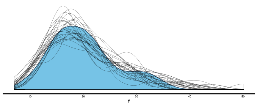
Random Forests ™ are a subset of the broader group of ensemble tree techniques known as “random decision forests”, and I set out to explore one variant of random decision forests visually (I’m a very visual person – if I can’t make a picture or movie of something happening I can’t understand it). The animation below shows an ensemble of 50 differing trees, where each tree was fitted to a set of data sample with replacement from the original data, and each tree was also restricted to just three randomly chosen variables. Note that this differs from a Random Forest, where the restriction differs for each split within a tree, rather than being a restriction for the tree as a whole.

Image may be NSFW.
Clik here to view.

Here’s how I generated my spinney of regression trees. Some of this code depends on a particular folder structure. The basic strategy is to

  • work out which variables have the most crude explanatory power
  • subset the data
  • subset the variables, choosing those with good explanatory power more often than the weaker ones
  • use cross-validation to work out the best tuning for the complexity parameter
  • fit the best tree possible with our subset of data nad variables
  • draw an image, with appropriate bits of commentary and labelling added to it, and save it for later
  • repeat the above 50 times, and then knit all the images into an animated GIF using ImageMagick.
#----------home made random decision forest--------------
# resample both rows and columns, as in a random decision forest,
# and draw a picture for each fitted tree.  Knit these
# into an animation.  Note this isn't quite the same as a random forest (tm).

# define the candidate variables
variables <- c("sex", "agegrp", "occupation", "qualification",
               "region", "hours", "Maori")

# estimate the value of the individual variables, one at a time

var_weights <- data_frame(var = variables, r2 = 0)
for(i in 1:length(variables)){
   tmp <- trainData[ , c("income", variables[i])]
   if(variables[i] == "hours"){
      tmp$hours <- sqrt(tmp$hours)
   }
   tmpmod <- lm(income ~ ., data = tmp)
   var_weights[i, "r2"] <- summary(tmpmod)$adj.r.squared
}

svg("..http://ellisp.github.io/img/0026-variables.svg", 8, 6)
print(
   var_weights %>%
   arrange(r2) %>%
   mutate(var = factor(var, levels = var)) %>%
   ggplot(aes(y = var, x = r2)) +
   geom_point() +
   labs(x = "Adjusted R-squared from one-variable regression",
        y = "",
        title = "Effectiveness of one variable at a time in predicting income")
)
dev.off()


n <- nrow(trainData)

home_made_rf <- list()
reps <- 50

commentary <- str_wrap(c(
   "This animation illustrates the use of an ensemble of regression trees to improve estimates of income based on a range of predictor variables.",
   "Each tree is fitted on a resample with replacement from the original data; and only three variables are available to the tree.",
   "The result is that each tree will have a different but still unbiased forecast for a new data point when a prediction is made.  Taken together, the average prediction is still unbiased and has less variance than the prediction of any single tree.",
   "This method is similar but not identical to a Random Forest (tm).  In a Random Forest, the choice of variables is made at each split in a tree rather than for the tree as a whole."
   ), 50)


set.seed(123)
for(i in 1:reps){
   
   these_variables <- sample(var_weights$var, 3, replace = FALSE, prob = var_weights$r2)
   
   this_data <- trainData[
      sample(1:n, n, replace = TRUE),
      c(these_variables, "income")
   ]


   this_rpartTune <- train(this_data[,1:3], this_data[,4],
                      method = "rpart",
                      tuneLength = 10,
                      trControl = trainControl(method = "cv"))


   home_made_rf[[i]] <- rpart(income ~ ., data = this_data, 
                      control = rpart.control(cp = this_rpartTune$bestTune),
                      method = "anova")
 
   png(paste0("_output/0026_random_forest/", 1000 + i, ".png"), 1200, 1000, res = 100)  
      par(fg = "blue", family = "myfont")
      prp(home_made_rf[[i]], varlen = 5, faclen = 7, type = 4, extra = 1, 
          under = TRUE, tweak = 0.9, box.col = "grey95", border.col = "grey92",
          split.font = 1, split.cex = 0.8, eq = ": ", facsep = " ",
          branch.col = "grey85", under.col = "lightblue",
          node.fun = node.fun1, mar = c(3, 1, 5, 1))
      
      grid.text(paste0("Variables available to this tree: ", 
                      paste(these_variables, collapse = ", "))
                , 0.5, 0.90,
                gp = gpar(fontfamily = "myfont", cex = 0.8, col = "darkblue"))
      
      grid.text("One tree in a random spinney - three randomly chosen predictor variables for weekly income,
resampled observations from New Zealand Income Survey 2011", 0.5, 0.95,
                gp = gpar(fontfamily = "myfont", cex = 1))
      
      grid.text(i, 0.05, 0.05, gp = gpar(fontfamily = "myfont", cex = 1))
      
      grid.text("$ numbers in blue are 'average' weekly income:nsquared(mean(sign(sqrt(abs(x)))))nwhich is a little less than the median.",
                0.8, 0.1, 
                gp = gpar(fontfamily = "myfont", cex = 0.8, col = "blue"))
      
      comment_i <- floor(i / 12.5) + 1
      
      grid.text(commentary[comment_i], 
                0.3, 0.1,
                gp = gpar(fontfamily = "myfont", cex = 1.2, col = "orange"))
      
      dev.off()

}   

# knit into an actual animation
old_dir <- setwd("_output/0026_random_forest")
# combine images into an animated GIF
system('"C:\Program Files\ImageMagick-6.9.1-Q16\convert" -loop 0 -delay 400 *.png "rf.gif"') # Windows
# system('convert -loop 0 -delay 400 *.png "rf.gif"') # linux
# move the asset over to where needed for the blog
file.copy("rf.gif", "../../..http://ellisp.github.io/img/0026-rf.gif", overwrite = TRUE)
setwd(old_dir)

Random Forest

Next model to try is a genuine Random Forest ™. As mentioned above, a Random Forest is an ensemble of regression trees, where each tree is a resample with replacement (variations are possible) of the original data, and each split in the tree is only allowed to choose from a subset of the variables available. To do this I used the {randomForests} R package, but it’s not efficiently written and is really pushing its limits with data of this size on modest hardware like mine. For classification problems the amazing open source H2O (written in Java but binding nicely with R) gives super-efficient and scalable implementations of Random Forests and of deep learning neural networks, but it doesn’t work with a continuous response variable.

Training a Random Forest requires you to specify how many explanatory variables to make available for each individual tree, and the best way to decide this is vai cross validation.

Cross-validation is all about splitting the data into a number of different training and testing sets, to get around the problem of using a single hold-out test set for multiple purposes. It’s better to give each bit of the data a turn as the hold-out test set. In the tuning exercise below, I divide the data into ten so I can try different values of the “mtry” parameter in my randomForest fitting and see the average Root Mean Square Error for the ten fits for each value of mtry. “mtry” defines the number of variables the tree building algorithm has available to it at each split of the tree. For forests with a continuous response variable like mine, the default value is the number of variables divided by three and I have 10 variables, so I try a range of options from 2 to 6 as the subset of variables for the tree to choose from at each split. It turns out the conventional default value of mtry = 3 is in fact the best:

Image may be NSFW.
Clik here to view.
rf-tuning

Here’s the code for this home-made cross-validation of randomForest:

#-----------------random forest----------
# Hold ntree constant and try different values of mtry
# values of m to try for mtry for cross-validation tuning
m <- c(1, 2, 3, 4, 5, 6)

folds <- 10

cvData <- trainData %>%
   mutate(group = sample(1:folds, nrow(trainData), replace = TRUE))

results <- matrix(numeric(length(m) * folds), ncol = folds)


# Cross validation, done by hand with single processing - not very efficient or fast:
for(i in 1:length(m)){
   message(i)
   for(j in 1:folds){
      
      cv_train <- cvData %>% filter(group != j) %>% select(-group)
      cv_test <- cvData %>% filter(group == j) %>% select(-group)

      tmp <- randomForest(income ~ ., data = cv_train, ntree = 100, mtry = m[i], 
                          nodesize = 10, importance = FALSE, replace = FALSE)
      tmp_p <- predict(tmp, newdata = cv_test)
      
      results[i, j] <- RMSE(tmp_p, cv_test$income)
      print(paste("mtry", m[i], j, round(results[i, j], 2), sep = " : "))
   }
}

results_df <- as.data.frame(results)
results_df$mtry <- m

svg("..http://ellisp.github.io/img/0026-rf-cv.svg", 6, 4)
print(
   results_df %>% 
   gather(trial, RMSE, -mtry) %>% 
   ggplot() +
   aes(x = mtry, y = RMSE) +
   geom_point() +
   geom_smooth(se = FALSE) +
   ggtitle(paste0(folds, "-fold cross-validation for random forest;ndiffering values of mtry"))
)
dev.off()

Having determined a value for mtry of three variables to use for each tree in the forest, we re-fit the Random Forest with the full training dataset. It’s interesting to see the “importance” of the different variables – which ones make the most contribution to the most trees in the forest. This is the best way of relating as Random Forest to a theoretical question; otherwise their black box nature makes them harder to interpret than a more traditional regression with its t tests and confidence intervals for each explanatory variable’s explanation.

It’s also good to note that after the first 300 or so trees, increasing the size of the forest seems to have little impact.

Image may be NSFW.
Clik here to view.
final-forest

Here’s the code that fits this forest to the training data and draws those plots:

# refit model with full training data set
rf <- randomForest(income ~ ., 
                    data = trainData, 
                    ntrees = 500, 
                    mtries = 3,
                    importance = TRUE,
                    replace = FALSE)


# importances
ir <- as.data.frame(importance(rf))
ir$variable  <- row.names(ir)

p1 <- ir %>%
   arrange(IncNodePurity) %>%
   mutate(variable = factor(variable, levels = variable)) %>%
   ggplot(aes(x = IncNodePurity, y = variable)) + 
   geom_point() +
   labs(x = "Importance of contribution tonestimating income", 
        title = "Variables in the random forest")

# changing RMSE as more trees added
tmp <- data_frame(ntrees = 1:500, RMSE = sqrt(rf$mse))
p2 <- ggplot(tmp, aes(x = ntrees, y = RMSE)) +
   geom_line() +
   labs(x = "Number of trees", y = "Root mean square error",
        title = "Improvement in predictionnwith increasing number of trees")

grid.arrange(p1, p2, ncol = 2)

Extreme gradient boosting

I wanted to check out extreme gradient boosting as an alternative prediction method. Like Random Forests, this method is based on a forest of many regression trees, but in the case of boosting each tree is relatively shallow (not many layers of branch divisions), and the trees are not independent of eachother. Instead, successive trees are built specifically to explain the observations poorly explained by previous trees – this is done by giving extra weight to outliers from the prediction to date.

Boosting is prone to over-fitting and if you let it run long enough it will memorize the entire training set (and be useless for new data), so it’s important to use cross-validation to work out how many iterations are worth using and at what point is not picking up general patterns but just the idiosyncracies of the training sample data. The excellent {xgboost} R package by Tianqui Chen, Tong He and Michael Benesty applies gradient boosting algorithms super-efficiently and comes with built in cross-validation functionality. In this case it becomes clear that 15 or 16 rounds is the maximum boosting before overfitting takes place, so my final boosting model is fit to the full training data set with that number of rounds.

#-------xgboost------------
sparse_matrix <- sparse.model.matrix(income ~ . -1, data = trainData)

# boosting with different levels of rounds.  After 16 rounds it starts to overfit:
xgb.cv(data = sparse_matrix, label = trainY, nrounds = 25, objective = "reg:linear", nfold = 5)

mod_xg <- xgboost(sparse_matrix, label = trainY, nrounds = 16, objective = "reg:linear")

Two stage Random Forests

My final serious candidate for a predictive model is a two stage Random Forest. One of my problems with this data is the big spike at $0 income per week, and this suggests a possible way of modelling it does so in two steps:

  • first, fit a classification model to predict the probability of an individual, based on their characteristics, having any income at all
  • fit a regression model, conditional on them getting any income and trained only on those observations with non-zero income, to predict the size of their income (which may be positive or negative).

The individual models could be chosen from many options but I’ve opted for Random Forests in both cases. Because the first stage is a classification problem, I can use the more efficient H2O platform to fit it – much faster.

#---------------------two stage approach-----------
# this is the only method that preserves the bimodal structure of the response
# Initiate an H2O instance that uses 4 processors and up to 2GB of RAM
h2o.init(nthreads = 4, max_mem_size = "2G")

var_names <- names(trainData)[!names(trainData) == "income"]

trainData2 <- trainData %>%
   mutate(income = factor(income != 0)) %>%
   as.h2o()

mod1 <- h2o.randomForest(x = var_names, y = "income",
                         training_frame = trainData2,
                         ntrees = 1000)

trainData3 <- trainData %>% filter(income != 0) 
mod2 <- randomForest(income ~ ., 
                     data = trainData3, 
                     ntree = 250, 
                     mtry = 3, 
                     nodesize = 10, 
                     importance = FALSE, 
                     replace = FALSE)

Traditional regression methods

As a baseline, I also fit three more traditional linear regression models:

  • one with all variables
  • one with all variables and many of the obvious two way interactions
  • a stepwise selection model.

I’m not a big fan of stepwise selection for all sorts of reasons but if done carefully, and you refrain from interpreting the final model as though it was specified in advance (which virtually everyone gets wrong) they have their place. It’s certainly a worthwhile comparison point as stepwise selection still prevails in many fields despite development in recent decades of much better methods of model building.

Here’s the code that fit those ones:

#------------baseline linear models for reference-----------
lin_basic <- lm(income ~ sex + agegrp + occupation + qualification + region +
                   sqrt(hours) + Asian + European + Maori + MELAA + Other + Pacific + Residual, 
                data = trainData)          # first order only
lin_full  <- lm(income ~ (sex + agegrp + occupation + qualification + region +
                   sqrt(hours) + Asian + European + Maori + MELAA + Other + Pacific + Residual) ^ 2, 
                data = trainData)  # second order interactions and polynomials
lin_fullish <- lm(income ~ (sex + Maori) * (agegrp + occupation + qualification + region +
                     sqrt(hours)) + Asian + European + MELAA + 
                     Other + Pacific + Residual,
                  data = trainData) # selected interactions only

lin_step <- stepAIC(lin_fullish, k = log(nrow(trainData))) # bigger penalisation for parameters given large dataset

Results – predictive power

I used root mean square error of the predictions of (transformed) income in the hold-out test set – which had not been touched so far in the model-fitting – to get an assessment of how well the various methods perform. The results are shown in the plot below. Extreme gradient boosting and my two stage Random Forest approaches are neck and neck, followed by the single tree and the random decision forest, with the traditional linear regressions making up the “also rans”.

Image may be NSFW.
Clik here to view.
rmses

I was surprised to see that a humble single regression tree out-performed my home made random decision forest, but concluded that this is probably something to do with the relatively small number of explanatory variables to choose from, and the high performance of “hours worked” and “occupation” in predicting income. A forest (or spinney…) that excludes those variables from whole trees at a time will be dragged down by trees with very little predictive power. In contrast, Random Forests choose from a random subset of variables at each split, so excluding hours from the choice in one split doesn’t deny it to future splits in the tree, and the tree as a whole still makes a good contribution.

It’s useful to compare at a glance the individual-level predictions of all these different models on some of the hold-out set, and I do this in the scatterplot matrix below. The predictions from different models are highly correlated with eachother (correlation of well over 0.9 in all cases), and less strongly correlated with the actual income. This difference is caused by the fact that the observed income includes individual level random variance, whereas all the models are predicting some kind of centre value for income given the various demographic values. This is something I come back to in the next stage, when I want to predict a full distribution.

Image may be NSFW.
Clik here to view.
pairs

Here’s the code that produces the predicted values of all the models on the test set and produces those summary plots:

#---------------compare predictions on test set--------------------
# prediction from tree
tree_preds <- predict(rpartTree, newdata = testData)

# prediction from the random decision forest
rdf_preds <- rep(NA, nrow(testData))
for(i in 1:reps){
   tmp <- predict(home_made_rf[[i]], newdata = testData)
   rdf_preds <- cbind(rdf_preds, tmp)
}
rdf_preds <- apply(rdf_preds, 1, mean, na.rm= TRUE)

# prediction from random forest
rf_preds <- as.vector(predict(rf, newdata = testData))

# prediction from linear models
lin_basic_preds <- predict(lin_basic, newdata = testData)
lin_full_preds <- predict(lin_full, newdata = testData)
lin_step_preds <-  predict(lin_step, newdata = testData)

# prediction from extreme gradient boosting
xgboost_pred <- predict(mod_xg, newdata = sparse.model.matrix(income ~ . -1, data = testData))

# prediction from two stage approach
prob_inc <- predict(mod1, newdata = as.h2o(select(testData, -income)), type = "response")[ , "TRUE"]
pred_inc <- predict(mod2, newdata = testData)
pred_comb <- as.vector(prob_inc > 0.5)  * pred_inc
h2o.shutdown(prompt = F) 

rmse <- rbind(
   c("BasicLinear", RMSE(lin_basic_preds, obs = testY)), # 21.31
   c("FullLinear", RMSE(lin_full_preds, obs = testY)),  # 21.30
   c("StepLinear", RMSE(lin_step_preds, obs = testY)),  # 21.21
   c("Tree", RMSE(tree_preds, obs = testY)),         # 20.96
   c("RandDecForest", RMSE(rdf_preds, obs = testY)),       # 21.02 - NB *worse* than the single tree!
   c("randomForest", RMSE(rf_preds, obs = testY)),        # 20.85
   c("XGBoost", RMSE(xgboost_pred, obs = testY)),    # 20.78
   c("TwoStageRF", RMSE(pred_comb, obs = testY))       # 21.11
   )

rmse %>%
   as.data.frame(stringsAsFactors = FALSE) %>%
   mutate(V2 = as.numeric(V2)) %>%
   arrange(V2) %>%
   mutate(V1 = factor(V1, levels = V1)) %>%
   ggplot(aes(x = V2, y = V1)) +
   geom_point() +
   labs(x = "Root Mean Square Error (smaller is better)",
        y = "Model type",
        title = "Predictive performance on hold-out test set of different models of individual income")

#------------comparing results at individual level------------
pred_results <- data.frame(
   BasicLinear = lin_basic_preds,
   FullLinear = lin_full_preds,
   StepLinear = lin_step_preds,
   Tree = tree_preds,
   RandDecForest = rdf_preds,
   randomForest = rf_preds,
   XGBoost = xgboost_pred,
   TwoStageRF = pred_comb,
   Actual = testY
)

pred_res_small <- pred_results[sample(1:nrow(pred_results), 1000),]

ggpairs(pred_res_small)

Building the Shiny app

There’s a few small preparatory steps now before I can put the results of my model into an interactive web app, which will be built with Shiny.

I opt for the two stage Random Forest model as the best way of re-creating the income distribution. It will let me create simulated data with a spike at zero dollars of income in a way none of the other models (which focus just on averages) will do; plus it has equal best (with extreme gradient boosting) in overall predictive power.

Adding back in individual level variation

After refitting my final model to the full dataset, my first substantive problem is to recreate the full distribution, with individual level randomness, not just a predicted value at each point. On my transformed scale for income, the residuals from the models are fairly homoskedastic, so decide that the Shiny app will simulate a population at any point by sampling with replacement from the residuals of the second stage model.

I save the models, the residauals, and the various dimension variables for my Shiny app.

#----------------shiny app-------------
# dimension variables for the user interface:
d_sex <- sort(as.character(unique(nzis$sex)))
d_agegrp <- sort(as.character(unique(nzis$agegrp)))
d_occupation <- sort(as.character(unique(nzis$occupation)))
d_qualification <- sort(as.character(unique(nzis$qualification)))
d_region <- sort(as.character(unique(nzis$region)))

save(d_sex, d_agegrp, d_occupation, d_qualification, d_region,
     file = "_output/0026-shiny/dimensions.rda")

# tidy up data of full dataset, combining various ethnicities into an 'other' category:     
nzis_shiny <- nzis %>% 
   select(-use) %>%
   mutate(Other = factor(ifelse(Other == "Yes" | Residual == "Yes" | MELAA == "Yes",
                         "Yes", "No"))) %>%
   select(-MELAA, -Residual)
   
for(col in c("European", "Asian", "Maori", "Other", "Pacific")){
   nzis_shiny[ , col]   <- ifelse(nzis_shiny[ , col] == "Yes", 1, 0)
   }

# Refit the models to the full dataset
# income a binomial response for first model
nzis_rf <- nzis_shiny %>%  mutate(income = factor(income !=0))
mod1_shiny <- randomForest(income ~ ., data = nzis_rf,
                           ntree = 500, importance = FALSE, mtry = 3, nodesize = 5)
save(mod1_shiny, file = "_output/0026-shiny/mod1.rda")

nzis_nonzero <- subset(nzis_shiny, income != 0) 

mod2_shiny <- randomForest(income ~ ., data = nzis_nonzero, ntree = 500, mtry = 3, 
                           nodesize = 10, importance = FALSE, replace = FALSE)

res <- predict(mod2_shiny) - nzis_pos$income
nzis_skeleton <- nzis_shiny[0, ]
all_income <- nzis$income

save(mod2_shiny, res, nzis_skeleton, all_income, nzis_shiny,
   file = "_output/0026-shiny/models.rda")

Contextual information – how many people are like “that” anyway?

After my first iteration of the web app, I realised that it could be badly misleading by giving a full distribution for a non-existent combination of demographic variables. For example, Maori female managers aged 15-19 with Bachelor or Higher qualification and living in Southland (predicted to have median weekly income of $932 for what it’s worth).

I realised that for meaningful context I needed a model that estimated the number of people in New Zealand with the particular combination of demographics selected. This is something that traditional survey estimation methods don’t provide, because individuals in the sample are weighted to represent a discrete number of exactly similar people in the population; there’s no “smoothing” impact allowing you to widen inferences to similar but not-identical people.

Fortunately this problem is simpler than the income modelling problem above and I use a straightforward generalized linear model with a Poisson response to create the seeds of such a model, with smoothed estimates of the number of people for each combination of demographics. I then can use iterative proportional fitting to force the marginal totals for each explanatory variable to match the population totals that were used to weight the original New Zealand Income Survey. Explaining this probably deserves a post of its own, but no time for that now.

#---------------population--------

nzis_pop <- expand.grid(d_sex, d_agegrp, d_occupation, d_qualification, d_region,
                        c(1, 0), c(1, 0), c(1, 0), c(1, 0), c(1, 0))
names(nzis_pop) <-  c("sex", "agegrp", "occupation", "qualification", "region",
                      "European", "Maori", "Asian", "Pacific", "Other")
nzis_pop$count <- 0
for(col in c("European", "Asian", "Maori", "Other", "Pacific")){
 nzis_pop[ , col]   <- as.numeric(nzis_pop[ , col])
}

nzis_pop <- nzis_shiny %>%
   select(-hours, -income) %>%
   mutate(count = 1) %>%
   rbind(nzis_pop) %>%
   group_by(sex, agegrp, occupation, qualification, region, 
             European, Maori, Asian, Pacific, Other) %>%
   summarise(count = sum(count)) %>%
   ungroup() %>%
   mutate(Ethnicities = European + Maori + Asian + Pacific + Other) %>%
   filter(Ethnicities %in% 1:2) %>%
   select(-Ethnicities)

# this pushes my little 4GB of memory to its limits:
 mod3 <- glm(count ~ (sex + Maori) * (agegrp + occupation + qualification) + region + 
                Maori:region + occupation:qualification + agegrp:occupation +
                agegrp:qualification, 
             data = nzis_pop, family = poisson)
 
 nzis_pop$pop <- predict(mod3, type = "response")

# total population should be (1787 + 1410) * 1000 = 319700.  But we also want
# the marginal totals (eg all men, or all women) to match the sum of weights
# in the NZIS (where wts = 319700 / 28900 = 1174).  So we use the raking method
# for iterative proportional fitting of survey weights

wt <- 1174

sex_pop <- nzis_shiny %>%
   group_by(sex) %>%
   summarise(freq = length(sex) * wt)

agegrp_pop <- nzis_shiny %>%
   group_by(agegrp) %>%
   summarise(freq = length(agegrp) * wt)

occupation_pop <- nzis_shiny %>%
   group_by(occupation) %>%
   summarise(freq = length(occupation) * wt)

qualification_pop <- nzis_shiny %>%
   group_by(qualification) %>%
   summarise(freq = length(qualification) * wt)

region_pop <- nzis_shiny %>%
   group_by(region) %>%
   summarise(freq = length(region) * wt)

European_pop <- nzis_shiny %>%
   group_by(European) %>%
   summarise(freq = length(European) * wt)

Asian_pop <- nzis_shiny %>%
   group_by(Asian) %>%
   summarise(freq = length(Asian) * wt)

Maori_pop <- nzis_shiny %>%
   group_by(Maori) %>%
   summarise(freq = length(Maori) * wt)

Pacific_pop <- nzis_shiny %>%
   group_by(Pacific) %>%
   summarise(freq = length(Pacific) * wt)

Other_pop <- nzis_shiny %>%
   group_by(Other) %>%
   summarise(freq = length(Other) * wt)

nzis_svy <- svydesign(~1, data = nzis_pop, weights = ~pop)

nzis_raked <- rake(nzis_svy,
                   sample = list(~sex, ~agegrp, ~occupation, 
                                 ~qualification, ~region, ~European,
                                 ~Maori, ~Pacific, ~Asian, ~Other),
                   population = list(sex_pop, agegrp_pop, occupation_pop,
                                     qualification_pop, region_pop, European_pop,
                                     Maori_pop, Pacific_pop, Asian_pop, Other_pop),
                   control = list(maxit = 20, verbose = FALSE))

nzis_pop$pop <- weights(nzis_raked)

save(nzis_pop, file = "_output/0026-shiny/nzis_pop.rda")

The final shiny app

To leave a comment for the author, please follow the link and comment on their blog: Peter's stats stuff - R.

R-bloggers.com offers daily e-mail updates about R news and tutorials on topics such as: Data science, Big Data, R jobs, visualization (ggplot2, Boxplots, maps, animation), programming (RStudio, Sweave, LaTeX, SQL, Eclipse, git, hadoop, Web Scraping) statistics (regression, PCA, time series, trading) and more...

11 new R jobs from around the world (2016-01-25)

This is the bi-monthly R-bloggers post (for 2016-01-25) for new R Jobs.

To post your R job on the next post

Just visit this link and post a new R job to the R community (it’s free and quick).

New R jobs

  1. Freelance
    R Analytics Consultant
    Evergreen Retail – Posted by EvergreenRetail
    Anywhere
    24 Jan2016
  2. Full-Time
    R Programming Software Engineer III @ Princeton, New Jersey USA
    sdemaree
    Princeton
    New Jersey, United States
    24 Jan2016
  3. Full-Time
    Internship at Genentech @ South San Francisco, California, U.S.
    Genentech – Posted by FabioB
    South San Francisco
    California, United States
    20 Jan2016
  4. Full-Time
    Postdoctoral Teaching & Learning Fellow
    University of British Columbia – Posted by Jennifer (Jenny) Bryan
    Vancouver
    British Columbia, Canada
    20 Jan2016
  5. Freelance
    Seeking a R developer with Shiny experience
    Crowdfundmarkt – Posted by crowdfundmarkt
    Anywhere
    19 Jan2016
  6. Full-Time
    Research Scientist in Johns Hopkins University @ Baltimore, Maryland, U.S.
    The Johns Hopkins University – Posted by The Johns Hopkins University
    Baltimore
    Maryland, United States
    17 Jan2016
  7. Full-Time
    Statistician / Data Analyst @ Watermael-Boitsfort, Bruxelles, Belgium
    International Diabetes Federation – Posted by Lydia Elizabeth Makaroff
    Watermael-Boitsfort
    Bruxelles, Belgium
    17 Jan2016
  8. Freelance
    Seeking a R-Developer with RCharts & Shiny Experience
    tgriggs202
    Anywhere
    16 Jan2016
  9. Full-Time
    Data Scientist – DMP @ București, Romania
    Quantum Data Science – Posted by Lucia Maria Ciuca
    București
    Municipiul București, Romania
    14 Jan2016
  10. Full-Time
    Data Engineer / Scientist at Zapier
    Zapier – Posted by mikeknoop
    Anywhere
    13 Jan2016
  11. Full-Time
    Senior Statistician @ Broughton, England
    JBA Risk ManagementLimited – Posted byye.liu@jbarisk.com
    BroughtonEngland, United Kingdom
    12 Jan2016


Job seekers: please follow the links below to learn more and apply for your job of interest:

(In R-users.com you may see all the R jobs that are currently available)

Image may be NSFW.
Clik here to view.
r_jobs

(you may also look at previous R jobs posts).

Bayesian regression with STAN Part 2: Beyond normality

(This article was first published on DataScience+, and kindly contributed to R-bloggers)

In a previous post we saw how to perform bayesian regression in R using STAN for normally distributed data. In this post we will look at how to fit non-normal model in STAN using three example distributions commonly found in empirical data: negative-binomial (overdispersed poisson data), gamma (right-skewed continuous data) and beta-binomial (overdispersed binomial data).

The STAN code for the different models is at the end of this posts together with some explanations.

Negative Binomial

The Poisson distribution is a common choice to model count data, it assumes that the variance is equal to the mean. When the variance is larger than the mean, the data are said to be overdispersed and the Negative Binomial distribution can be used. Say we have measured a response variable y that follow a negative binomial distribution and depends on a set of k explanatory variables X, in equation this gives us:
$$ y_{i} sim NB(mu_{i},phi) $$ $$ E(y_{i}) = mu_{i} $$ $$ Var(y_{i}) = mu_{i} + mu_{i}^{2} / phi $$ $$ log(mu_{i}) = beta_{0} + beta_{1} * X1_{i} + … + beta_{k} * Xk_{i} $$
The negative binomial distribution has two parameters: (mu) is the expected value that need to be positive, therefore a log link function can be used to map the linear predictor (the explanatory variables times the regression parameters) to (mu) (see the 4th equation); and (phi) is the overdispersion parameter, a small value means a large deviation from a Poisson distribution, while as (phi) gets larger the negative binomial looks more and more like a Poisson distribution.

Let’s simulate some data and fit a STAN model to them:

#load the libraries
library(arm) #for the invlogit function
library(emdbook) #for the rbetabinom function
library(rstan)
library(rstanarm) #for the launch_shinystan function

#simulate some negative binomial data
#the explanatory variables
N<-100 #sample size
dat<-data.frame(x1=runif(N,-2,2),x2=runif(N,-2,2))
#the model
X<-model.matrix(~x1*x2,dat)
K<-dim(X)[2] #number of regression params
#the regression slopes
betas<-runif(K,-1,1)
#the overdispersion for the simulated data
phi<-5
#simulate the response
y_nb<-rnbinom(100,size=phi,mu=exp(X%*%betas))

#fit the model
m_nb<-stan(file = "neg_bin.stan",data = list(N=N,K=K,X=X,y=y_nb),pars=c("beta","phi","y_rep"))

#diagnose and explore the model using shinystan
launch_shinystan(m_nb)

Shinystan:
Image may be NSFW.
Clik here to view.
stan_glm0

The last command should open a window in your browser with loads of options to diagnose, estimate and explore your model. Some options are beyond my limited knowledge (ie Log Posterior vs Sample Step Size), so I usually look at the posterior distribution of the regression parameters (Diagnose -> NUTS (plots) -> By model parameter), the histogram should be more or less normal. I also look at Posterior Predictive Checks (Diagnose -> PPcheck -> Distribution of observed data vs replications), the distribution of the y_rep should be equivalent to the observed data.

The model looks fine, we can now plot the predicted regression lines with their credible intervals using the sampled regression parameters from the model:

#get the posterior predicted values together with the credible intervals 
post<-as.array(m_nb) #the sampled model values
#will look at varying x2 with 3 values of x1
new_X<-model.matrix(~x1*x2,expand.grid(x2=seq(-2,2,length=10),x1=c(min(dat$x1),mean(dat$x1),max(dat$x1))))
#get the predicted values for each samples
pred<-apply(post[,,1:4],c(1,2),FUN = function(x) new_X%*%x)
#each chains is in a different matrix re-group the info into one matrix
dim(pred)<-c(30,4000)
#get the median prediction plus 95% credible intervals
pred_int<-apply(pred,1,quantile,probs=c(0.025,0.5,0.975))

#plot
plot(dat$x2,y_nb,pch=16)
lines(new_X[1:10,3],exp(pred_int[2,1:10]),col="orange",lwd=5)
lines(new_X[1:10,3],exp(pred_int[1,1:10]),col="orange",lwd=3,lty=2)
lines(new_X[1:10,3],exp(pred_int[3,1:10]),col="orange",lwd=3,lty=2)
lines(new_X[1:10,3],exp(pred_int[2,11:20]),col="red",lwd=5)
lines(new_X[1:10,3],exp(pred_int[1,11:20]),col="red",lwd=3,lty=2)
lines(new_X[1:10,3],exp(pred_int[3,11:20]),col="red",lwd=3,lty=2)
lines(new_X[1:10,3],exp(pred_int[2,21:30]),col="blue",lwd=5)
lines(new_X[1:10,3],exp(pred_int[1,21:30]),col="blue",lwd=3,lty=2)
lines(new_X[1:10,3],exp(pred_int[3,21:30]),col="blue",lwd=3,lty=2)
legend("topleft",legend=c("Min","Mean","Max"),ncol=3,col = c("orange","red","blue"),lwd = 3,bty="n",title="Value of x1")

Here it is the plot:
Image may be NSFW.
Clik here to view.
stan_glm1

As always with such models one must pay attention to the difference between the link and the response space. The model makes prediction in the link space, if we want to plot them next to the actual response value we need to apply the inverse of the link function (in our case exponentiate the values) to back-transform the model prediction.

Gamma distribution

Sometime we collect continuous data that show right-skew, like body sizes or plant biomass, such data may be modelled using a log-normal distribution (basically log-transforming the reponse) or using a gamma distribution (see this discussion). Here I will look at gamma distribution, say we collected some gamma-distributed y responding to some explanatory variable X, in equation this gives us:
$$ y_{i} sim Gamma(alpha,beta) $$ $$ E(y_{i}) = alpha / beta $$ $$ Var(y_{i}) = alpha / beta^{2} $$
Mmmmmmm in contrary to the negative binomial above we cannot directly map the linear predictor directly to one parameter of the model ((mu) for example). So we need to re-parametrize the model by doing some calculus:
$$ E(y_{i}) = alpha / beta = mu $$ $$ Var(y_{i}) = alpha / beta^{2} = phi $$
Re-arranging gives us:
$$ alpha = mu^{2} / phi $$ $$ beta = mu / phi $$
Where (mu) is now our expected value and (phi) a dispersion parameter like in the Negative Binomial example above. As (alpha) and (beta) must be positive we can use again a log link on the linear predictor:
$$ log(mu_{i}) = beta_{0} + beta_{1} * X1_{i} + … + beta_{k} * Xk_{i} $$
Let’s simulate some data and fit a model to this:

#simulate gamma data
mus<-exp(X%*%betas)
y_g<-rgamma(100,shape=mus**2/phi,rate=mus/phi)

#model
m_g<-stan(file = "gamma.stan",data = list(N=N,K=K,X=X,y=y_g),pars=c("betas","phi","y_rep"))

#model check
launch_shinystan(m_g)

Again we check that the model is correct, everything is very nice on this front. We can plot the results using similar code as above replacing m_nb by m_g. Since we used the same link function in the Negative Binomial and the Gamma model the rest will work.

Image may be NSFW.
Clik here to view.
stan_glm2

Beta-binomial

Finally when we collect data from a certain number of trials (I throw ten time a coin what is the proportion of heads?) the response usually follows a binomial distribution. Now empirical data are messy and just like Poisson data may be overdispersed, so can binomial be. To account for this the Beta-Binomial model can be used:
$$ y_{i} sim BetaBinomial(N,alpha,beta) $$ $$ E(y_{i}) = N*alpha / (alpha + beta) $$
Leaving the variance expression aside (have a look here to see how ugly it is), and the constant N (the number of trials), we can like in the Gamma example re-parametrize the equations to an expected value of (mu) and a dispersion parameter (phi):
$$ alpha = mu * phi $$ $$ beta = (1-mu) * phi $$
This time the (mu) represent a probability and must therefore be between 0 and 1, one can use the logit link to map the linear predictor to (mu):
$$ logit(mu) = beta_{0} + beta_{1} * X1_{i} + … + beta_{k} * Xk_{i} $$
Again simulation power:

#simulate beta-binomial data
W<-rep(20,100) #number of trials
y_bb<-rbetabinom(100,prob=invlogit(X%*%betas),size=W,theta=phi)

#model
m_bb<-stan(file = "beta_bin.stan",data = list(N=N,W=W,K=K,X=X,y=y_bb),pars=c("betas","phi","y_rep"))

#model check
launch_shinystan(m_bb)

Everything is great, we can now plot this:

#get the posterior predicted values together with the credible intervals 
post<-as.array(m_bb) #the posterior draw
#get the predicted values
pred<-apply(post[,,1:4],c(1,2),FUN = function(x) new_X%*%x)
#each chains is in a different matrix re-group the info
dim(pred)<-c(30,4000)
#get the median prediction plus 95% credible intervals
pred_int<-apply(pred,1,quantile,probs=c(0.025,0.5,0.975))

#plot
plot(dat$x2,y_bb,pch=16)
lines(new_X[1:10,3],20*invlogit(pred_int[2,1:10]),col="orange",lwd=5)
lines(new_X[1:10,3],20*invlogit(pred_int[1,1:10]),col="orange",lwd=3,lty=2)
lines(new_X[1:10,3],20*invlogit(pred_int[3,1:10]),col="orange",lwd=3,lty=2)
lines(new_X[1:10,3],20*invlogit(pred_int[2,11:20]),col="red",lwd=5)
lines(new_X[1:10,3],20*invlogit(pred_int[1,11:20]),col="red",lwd=3,lty=2)
lines(new_X[1:10,3],20*invlogit(pred_int[3,11:20]),col="red",lwd=3,lty=2)
lines(new_X[1:10,3],20*invlogit(pred_int[2,21:30]),col="blue",lwd=5)
lines(new_X[1:10,3],20*invlogit(pred_int[1,21:30]),col="blue",lwd=3,lty=2)
lines(new_X[1:10,3],20*invlogit(pred_int[3,21:30]),col="blue",lwd=3,lty=2)
legend("topleft",legend=c("Min","Mean","Max"),ncol=3,col = c("orange","red","blue"),lwd = 3,bty="n",title="Value of x1")

This is the plot:
Image may be NSFW.
Clik here to view.
stan_glm3

Note the change from exp to invlogit taking into account the different link function used.

Parting thoughts

In this post we saw how to adapt our models to non-normal data that are pretty common out there. STAN is very flexible and allow many different parametrization for many different distributions (see the reference guide), the possibilities are only limited by your hypothesis (and maybe a bit your mathematical skills …). At this point I’d like you to note that the rstanarm package allows you to fit STAN model without you having to write down the model. Instead using the typical R syntax one would use in, for example, a glm call (see this post). So why bothering learning all this STAN stuff? It depends: if you are only fitting “classical” models to your data with little fanciness then just use rstanarm this will save you some time to do your science and the models in this package are certainly better parametrized (ie faster) than the one I presented here. On the other hand if you feel that one day you will have to fit your own customized models then learning STAN is a good way to tap into a highly flexible and powerful language that will keep growing.

Model Code

Negative Binomial:


/*
*Simple negative binomial regression example
*using the 2nd parametrization of the negative
*binomial distribution, see section 40.1-3 in the Stan
*reference guide
*/

data {
  int N; //the number of observations
  int K; //the number of columns in the model matrix
  int y[N]; //the response
  matrix[N,K] X; //the model matrix
}
parameters {
  vector[K] beta; //the regression parameters
  real phi; //the overdispersion parameters
}
transformed parameters {
  vector[N] mu;//the linear predictor
  mu <- exp(X*beta); //using the log link 
}
model {  
  beta[1] ~ cauchy(0,10); //prior for the intercept following Gelman 2008

  for(i in 2:K)
   beta[i] ~ cauchy(0,2.5);//prior for the slopes following Gelman 2008
  
  y ~ neg_binomial_2(mu,phi);
}
generated quantities {
 vector[N] y_rep;
 for(n in 1:N){
  y_rep[n] <- neg_binomial_2_rng(mu[n],phi); //posterior draws to get posterior predictive checks
 }
}

Gamma:


/*
*Simple gamma example
*Note that I used a log link which makes
*more sense in most applied cases
*than the canonical inverse link
*/

data {
  int N; //the number of observations
  int K; //the number of columns in the model matrix
  real y[N]; //the response
  matrix[N,K] X; //the model matrix
}
parameters {
  vector[K] betas; //the regression parameters
  real phi; //the variance parameter
}
transformed parameters {
  vector[N] mu; //the expected values (linear predictor)
  vector[N] alpha; //shape parameter for the gamma distribution
  vector[N] beta; //rate parameter for the gamma distribution
  
  mu <- exp(X*betas); //using the log link 
  alpha <- mu .* mu / phi; 
  beta <- mu / phi;
}
model {  
  betas[1] ~ cauchy(0,10); //prior for the intercept following Gelman 2008

  for(i in 2:K)
   betas[i] ~ cauchy(0,2.5);//prior for the slopes following Gelman 2008
  
  y ~ gamma(alpha,beta);
}
generated quantities {
 vector[N] y_rep;
 for(n in 1:N){
  y_rep[n] <- gamma_rng(alpha[n],beta[n]); //posterior draws to get posterior predictive checks
 }
}

Beta-Binomial:


/*
*Simple beta-binomial example
*/

data {
  int N; //the number of observations
  int K; //the number of columns in the model matrix
  int y[N]; //the response
  matrix[N,K] X; //the model matrix
  int W[N]; //the number of trials per observations, ie a vector of 1 for a 0/1 dataset
}
parameters {
  vector[K] betas; //the regression parameters
  real phi; //the overdispersion parameter
}
transformed parameters {
  vector[N] mu; //the linear predictor
  vector[N] alpha; //the first shape parameter for the beta distribution
  vector[N] beta; //the second shape parameter for the beta distribution
  
  for(n in 1:N)
   mu[n] <- inv_logit(X[n,]*betas); //using logit link
  alpha <- mu * phi;
  beta <- (1-mu) * phi;
}
model {  
  betas[1] ~ cauchy(0,10); //prior for the intercept following Gelman 2008

  for(i in 2:K)
   betas[i] ~ cauchy(0,2.5);//prior for the slopes following Gelman 2008
  
  y ~ beta_binomial(W,alpha,beta);
}
generated quantities {
 vector[N] y_rep;
 for(n in 1:N){
  y_rep[n] <- beta_binomial_rng(W[n],alpha[n],beta[n]); //posterior draws to get posterior predictive checks
 }
}

This bring us to the end of the post, if you have any question leave a comment below.

To leave a comment for the author, please follow the link and comment on their blog: DataScience+.

R-bloggers.com offers daily e-mail updates about R news and tutorials on topics such as: Data science, Big Data, R jobs, visualization (ggplot2, Boxplots, maps, animation), programming (RStudio, Sweave, LaTeX, SQL, Eclipse, git, hadoop, Web Scraping) statistics (regression, PCA, time series, trading) and more...

Need any more reason to love R-Shiny? Here: you can even use Shiny to create simple games!

(This article was first published on Dean Attali's R Blog, and kindly contributed to R-bloggers)

Anyone who reads my blog posts knows by now that I’m very enthusiastic about Shiny (the web app framework for R – if you didn’t know what Shiny is then I suggest reading my previous post about it). One of my reasons for liking Shiny so much is that you can do so much more with it than what it was built for, and it’s fun to think of new useful uses for it. Well, my latest realization is that you can even make simple games quite easily, as the lightsouts package and its companion web app/game demonstrate! I’m actually currently on my way to San Francisco for the first ever Shiny conference, so this post comes at a great time.

First, some background. I was recently contacted by Daniel Barbosa who offered to hire me for a tiny project: write a solver for the Lights Out puzzle in R. After a few minutes of Googling I found out that Lights Out is just a simple puzzle game that can be solved mathematically. The game consists of a grid of lights that are either on or off, and clicking on any light will toggle it and its neighbours. The goal of the puzzle is to switch all the lights off.

Here is a simple visual that shows what happens when pressing a light on a 5×5 board:

Image may be NSFW.
Clik here to view.
Lights Out instructions

The cool thing about Lights Out is that, as I mentioned, it can be solved mathematically. In other words, given any Lights Out board, there are a few algorithms that can be used to find the set of lights that need to be clicked in order to turn all the lights off. So when Daniel asked me to implement a Lights Out solver in R, it really just meant to write a function that would take a Lights Out board as input (easily represented as a binary matrix with 0 = light off and 1 = light on) and implement the algorithm that would determine which lights to click on. It turns out that there are a few different methods to do this, and I chose the one that involves mostly linear algebra because it was the least confusing to me. (If you’re curious about the solving algorithm, you can view my code here.)

At the time of completing this solver function I was traveling but bedridden, so I thought “well, why not go the extra half mile and make a package out of this, so that the game is playable?”, which is exactly what I did. The next day, the lightsout package was born, and it was capable of letting users play a Lights Out game in the R console. You can see the README of the package to get more information on that.

At this point you can predict what happened next. “Why don’t I complete that mile and just write a small Shiny app that will use the gameplay logic from the package and wrap it in a graphical user interface? That way there’ll be an actual useful game, not just some 1980 text-based game that gives people nightmares.”

Since the game logic was already fully implemented, making a Shiny app that encapsulates the game logic was very easy. You can play the Shiny-based game online or by downloading the package and running lightsout::launch(). Here is a screenshot of the app:

Image may be NSFW.
Clik here to view.
Lights Out game

You can view the code for the Shiny app to convince yourself of how simple it is by looking in the package source code. It only took ~40 lines of Shiny UI code, ~100 lines of Shiny server code, a little bit of styling with CSS, and absolutely no JavaScript. Yep, the game was built entirely in R, with 0 JavaScript (although I did make heavy use of shinyjs).

While this “game” might not be very impressive, I think it’s still a nice accomplishment to know that it was fully developed in R-Shiny. More importantly, it serves as a simple proof-of-concept to show that Shiny can be leveraged to make simple web-based games if you already have the logic implemented in R.

Disclaimer: I realize this may not necessarily be super practical because R isn’t used for these kinds of applications, but if anyone ever writes a chess or connect4 or any similar logic game in R, then complementing it with a similar Shiny app might make sense.

To leave a comment for the author, please follow the link and comment on their blog: Dean Attali's R Blog.

R-bloggers.com offers daily e-mail updates about R news and tutorials on topics such as: Data science, Big Data, R jobs, visualization (ggplot2, Boxplots, maps, animation), programming (RStudio, Sweave, LaTeX, SQL, Eclipse, git, hadoop, Web Scraping) statistics (regression, PCA, time series, trading) and more...
Viewing all 673 articles
Browse latest View live