Quantcast
Channel: Search Results for “shiny”– R-bloggers
Viewing all 673 articles
Browse latest View live

Supplementing your R package with a Shiny app

$
0
0

(This article was first published on Dean Attali's R Blog, and kindly contributed to R-bloggers)

The R community is generally very fond of open-source-ness and the idea of releasing all code to the public. Writing packages has become such an easy experience now that Hadley's devtools is so powerful, and as a result there are new packages being released by useRs every single day.

A good package needs to have two things: useful functionality, and clear usage instructions. The former is a no-brainer, while the latter is what developers usually dread the most - the D-word (Documentation. Yikes.). Proper documentation is essential so that others will know what your package can do and how to do it. And with the use of Shiny, we now have another great tool we can use to showcase a package's capabilities.

Incorporating Shiny

In a nutshell, Shiny is a package that lets you run your R code as an interactive webpage. What this means for package developers is that you can have an interactive webpage that lets users experiment with your package and see what it can do before having to read through the potentially lengthy function documentations/vignette.

As an example, I recently released a package for adding marginal plots to ggplot2. You be the judge: after that one-sentence description of some functionality, would you rather go straight to the README, or see it in action first in a Shiny app online? I might be wrong, but I think it's useful to interactively see what the package can do.

Making a Shiny app doesn't necessarily always make sense for every package, but there are certainly many times when it can be a great addition to a package's "documentation". I think that if a new package has some functions that can be easily illustrated in a simple Shiny app, it's worth it to take the extra 1-2 hours to develop it. This way, a user who finds your package and isn't quite sure what to do with it can try the Shiny app to see whether or not this is the functionality they were looking for. You can have several Shiny apps, each showing the usage of a particular function, or one app that is representative of a whole package. Whatever makes the most sense. Of course, having a Shiny app is in no way a replacement to documentation, it's just a useful add-on.


There are two ways to complement a package with a Shiny app that shows its main usage. These two methods are NOT mutually exclusive; I personally do both of them together:

1. Host the Shiny app online

You can host your Shiny app somewhre that is publicly available, such as shinyapps.io or on your own Shiny Server. Then you can include a link in the package's README or vignette or function documentation that points to the Shiny app.

As an example, I host my own Shiny Server where I can host my Shiny apps, and whenever I release a new package, I include a link in the README to a demo app.

The advantage of doing this is that people can play aroud with your package before even downloading it.

2. Include the app in the package and add a function to launch it

I recommend including the source code of the Shiny app in your package, and having a function such as runExample() that will launch the app. Here are the steps to do this (I've learned a lot from looking at shiny::runExample source code - thanks RStudio):

First, add Shiny as a dependency in your DESCRIPTION file (preferably under the Suggests: field).

Then place your Shiny app folder under inst/shiny-examples/ and add an R file called runExample.R. The package's tree structure should look like this

- mypacakge
  |- inst
     |- shiny-examples
        |- myapp
           |- ui.R
           |- server.R
  |- R
     |- runExample.R
     |- ...
  |- DESCRIPTION
  |- ...

Your runExample.R will be simple - it will just look for the Shiny app and launch it

#' @export
runExample <- function() {
  appDir <- system.file("shiny-examples", "myapp", package = "mypackage")
  if (appDir == "") {
    stop("Could not find example directory. Try re-installing `mypackage`.", call. = FALSE)
  }

  shiny::runApp(appDir, display.mode = "normal")
}

Of course, don't forget to document this function! Now users can try out an app showcasing your package by running mypackage::runExample().

This method can easily support more than one Shiny app as well, simply place each app under inst/shiny-examples/ and change the runExample code to something like this

runExample <- function(example) {
  # locate all the shiny app examples that exist
  validExamples <- list.files(system.file("shiny-examples", package = "mypackage"))

  validExamplesMsg <-
    paste0(
      "Valid examples are: '",
      paste(validExamples, collapse = "', '"),
      "'")

  # if an invalid example is given, throw an error
  if (missing(example) || !nzchar(example) ||
      !example %in% validExamples) {
    stop(
      'Please run `runExample()` with a valid example app as an argument.n',
      validExamplesMsg,
      call. = FALSE)
  }

  # find and launch the app
  appDir <- system.file("shiny-examples", example, package = "mypackage")
  shiny::runApp(appDir, display.mode = "normal")
}

Now running runExample("myapp") will launch the "myapp" app, and running runExample() will generate a message telling the user what examples are allowed.

To leave a comment for the author, please follow the link and comment on his blog: Dean Attali's R Blog.

R-bloggers.com offers daily e-mail updates about R news and tutorials on topics such as: visualization (ggplot2, Boxplots, maps, animation), programming (RStudio, Sweave, LaTeX, SQL, Eclipse, git, hadoop, Web Scraping) statistics (regression, PCA, time series, trading) and more...

Introducing shinyjs: perform common JavaScript operations in Shiny apps using plain R code

$
0
0

(This article was first published on Dean Attali's R Blog, and kindly contributed to R-bloggers)

shinyjs is my second R package that managed to find its way past the CRAN review process. It lets you perform common useful JavaScript operations in Shiny applications without having to know any JavaScript.

Demos

You can check out a demo Shiny app that lets you play around with some of the functionality that shinyjs makes available, or have a look at a very basic Shiny app that uses shinyjs to enhance the user experience with very minimal and simple R code.

Availability

shinyjs is available through both CRAN (install.packages("shinyjs")) and GitHub (devtools::install_github("daattali/shinyjs")).

Motivation

Shiny is a fantastic R package provided by RStudio that lets you turn any R code into an interactive webpage. It's very powerful and one of the most useful packages in my opinion. But there are just a few simple pieces of functionality that I always find missing and I implement myself in my Shiny apps using JavaScript (JS) because it's either not supported natively by Shiny or it's just cleaner to do so. Simple things like showing/hiding elements, enabling/disabling a button, showing a popup message to the user, manipulating the CSS class or HTML content of an element, etc.

After noticing that I'm writing the same JS code in all my apps, and since making Shiny talk to JS is a bit tedious and annoying with all the message passing, I decided to just package it to make it easily reusable. Now I can simply call hide("panel") or disable("button"). I was lucky enough to have previous experience with JS so I knew how to achieve the results that I wanted, but for any Shiny developer who is not proficient in JS, hopefully this package will make it easy to extend the power of their Shiny apps.

Overview of main functions

  • show/hide/toggle - display or hide an element. There are arguments that control the animation as well, though animation is off by default.

  • hidden - initialize a Shiny tag as invisible (can be shown later with a call to show)

  • enable/disable/toggleState - enable or disable an input element, such as a button or a text input.

  • info - show a message to the user (using JavaScript's alert under the hood)

  • text - change the text/HTML of an element (using JavaScript's innerHTML under the hood)

  • onclick - run R code when an element is clicked. Was originally developed with the sole purpose of running a shinyjs function when an element is clicked, though any R code can be used.

  • addClass/removeClass/toggleClass - add or remove a CSS class from an element

  • inlineCSS - easily add inline CSS to a Shiny app

  • logjs - print a message to the JavaScript console (mainly used for debugging purposes)

Check out the demo Shiny app to see some of these in action, or install shinyjs and run shinyjs::runExample() to see more demo apps.

Basic use case - working example

You can view the final Shiny app developed in this simple example here.

Suppose we want to have a simple Shiny app that collects a user's basic information (name, age, company) and submits it, along with the time of submission. Here is a very simple implementation of such an app (nothing actually happens when the user "submits").

library(shiny)
shinyApp(
  ui = fluidPage(
    div(id = "myapp",
      h2("shinyjs demo"),
      textInput("name", "Name", ""),
      numericInput("age", "Age", 30),
      textInput("company", "Company", ""),
      p("Timestamp: ", span(date())),
      actionButton("submit", "Submit")
    )
  ),

  server = function(input, output) {
  }
)

Note that I generally don't like running Shiny apps like this and prefer to declare the UI and server separately, but I do it like this here for brevity.

Here is what that app would look like

Demo app

Now suppose we want to add a few features to the app to make it a bit more user-friendly. First we need to set up the app to use shinyjs with two small changes

  1. A call to useShinyjs() needs to be made in the Shiny app's UI. This is required to set up all the JavaScript and a few other things.

  2. The app's server needs to have the session parameter declared, ie. initialize the server as server(input, output, session) instead of server(input, output).

Here are 6 features we'll add to the app, each followed with the code to implement it using shinyjs:

1. The "Name" field is mandatory and thus the "Submit" button should not be enabled if there is no name

In the server portion, add the following code

observe({
  if (is.null(input$name) || input$name == "") {
    shinyjs::disable("submit")
  } else {
    shinyjs::enable("submit")
  }
})

2. The "Age" and "Company" fields are optional and we want to have the ability to hide that section of the form

First, we need to section off the "Age" and "Company" elements into their own section, so we surround them with a div

div(id = "advanced",
  numericInput("age", "Age", 30),
  textInput("company", "Company", "")
)

We also need to add a link in the UI that will be used to hide/show the section

a(id = "toggleAdvanced", "Show/hide advanced info")

Lastly, we need to tell Shiny to show/hide the section when the link is clicked by adding this code to the server

shinyjs::onclick("toggleAdvanced",
                  shinyjs::toggle(id = "advanced", anim = TRUE))

3. Similarly, since we don't really care about "Age" and "Company" too much, we want to hide them initially when the form loads

Simply surround the section we want to hide initially with shinyjs::hidden

shinyjs::hidden(
  div(id = "advanced",
    ...
))

4. The user should be able to update the "Timestamp" in case he spends way too long filling out the form (not very realistic here, and the timestamp should ideally be determined when the button is clicked, but it's good enough for illustration purposes)

First, we need to add an "Update" link to click on, and we need to give the element showing the time an id so that we can refer to it later when we want to change its contents.

To do that, replace p("Timestamp: ", span(date())) with

p("Timestamp: ", span(id = "time", date()), a(id = "update", "Update"))

Now we need to tell Shiny what to do when "Update" is clicked by adding this to the server

shinyjs::onclick("update", shinyjs::text("time", date()))

5. Some users may find it hard to read the small text in the app, so there should be an option to increase the font size

First, we need to add checkbox to the UI

checkboxInput("big", "Bigger text", FALSE)

In order to make the text bigger, we will use CSS. So let's add an appropriate CSS rule by adding this code to the UI

shinyjs::inlineCSS(list(.big = "font-size: 2em"))

Lastly, we want the text to be big or small depending on whether the checkbox is checked by adding this code to the server

observe({
  if (input$big) {
    shinyjs::addClass("myapp", "big")
  } else {
    shinyjs::removeClass("myapp", "big")
  }
})

6. Give the user a "Thank you" message upon submission

Simply add the following to the server

observe({
  if (input$submit > 0) {
    shinyjs::info("Thank you!")
  }
})

The final code looks like this

library(shiny)
shinyApp(
  ui = fluidPage(
    shinyjs::useShinyjs(),
    shinyjs::inlineCSS(list(.big = "font-size: 2em")),
    div(id = "myapp",
        h2("shinyjs demo"),
        checkboxInput("big", "Bigger text", FALSE),
        textInput("name", "Name", ""),
        a(id = "toggleAdvanced", "Show/hide advanced info", href = "#"),
        shinyjs::hidden(
          div(id = "advanced",
            numericInput("age", "Age", 30),
            textInput("company", "Company", "")
          )
        ),
        p("Timestamp: ",
          span(id = "time", date()),
          a(id = "update", "Update", href = "#")
        ),
        actionButton("submit", "Submit")
    )
  ),

  server = function(input, output, session) {
    observe({
      if (is.null(input$name) || input$name == "") {
        shinyjs::disable("submit")
      } else {
        shinyjs::enable("submit")
      }
    })

    shinyjs::onclick("toggleAdvanced",
                     shinyjs::toggle(id = "advanced", anim = TRUE))    

    shinyjs::onclick("update", shinyjs::text("time", date()))

    observe({
      if (input$big) {
        shinyjs::addClass("myapp", "big")
      } else {
        shinyjs::removeClass("myapp", "big")
      }
    })

    observe({
      if (input$submit > 0) {
        shinyjs::info("Thank you!")
      }
    })    
  }
)

You can view the final app here.

Altenatives using native Shiny

shiny::conditionalPanel vs shinyjs::hide/show/toggle/hidden

It is possible to achieve a similar behaviour to hide and show by using shiny::conditionalPanel, though I've experienced that using conditionalPanel often gets my UI to a messier state. I still use conditionalPanel sometimes for basic use cases, but when there is some logic involved in hiding/showing, I find it much easier to move that logic to the server and use hide/show. I also think it's generally a better idea to keep most of the logic in the server, and using conditionalPanel violates that rule.
Implementing the shinyjs::toggle or shinyjs::hidden behaviour with pure Shiny is also possible but it also results in messier and less intuitive code.

shiny::render* and shiny::update* vs shinyjs::text

The shinyjs::text function can be used to change the text inside an element by either overwriting it or appending to it. I mostly intended for this function to be used to change the text, though it can also be used to add HTML elements. There are many Shiny functions that allow you to change the text of an element. For example, renderText is used on a textOutput tag and updateTextInput is used on a textInput tag. These functions are useful, but sometimes I like to be able to just cange the text of a tag without having to know/specify exactly what it was declared in the UI. These functions also don't work on tags that are not defined as reactive, so if I just have a p(id = "time", date()) it would be impossible to change it. I also don't think it's possible to append rather than overwrite with Shiny, and you can't use HTML unless the element is declared as uiOutput or something similar.

There is something to be said about the fact that the pure Shiny functions are safer and more strict, but I personally like having the extra flexibility sometimes, even though the text function feels like it doesn't really follow Shiny's patterns. I still use the Shiny functions often, but I find text useful as well.

shiny::observeEvent vs shinyjs::onclick

The onclick function was initially written because I wanted a way to click on a button that will cause a section to show/hide, like so:

shinyjs::onclick("toggleLink", shinyjs::toggle("section"))

RStudio very recently published an article describing several design patterns for using buttons, and from that article I learned that I can do what I wanted with observeEvent:

observeEvent("input$toggleLink", shinyjs::toggle("section"))

When I first discovered this, I thought of removing the onclick function because it's not useful anymore, but then I realized there are differences that still make it useful. observeEvent responds to "event-like" reactive values, while onclick responds to a mouse click on an element. This means that observeEvent can be used for any input element (not only clickable things), but onclick can be used for responding to a click on any element, even if it is not an input tag. Another small feature I wanted to support is the ability to overwrite vs add the click handler (= R code to run on a click). This would not be used for most basic apps, but for more complex dynamic apps it might come in handy.

To leave a comment for the author, please follow the link and comment on his blog: Dean Attali's R Blog.

R-bloggers.com offers daily e-mail updates about R news and tutorials on topics such as: visualization (ggplot2, Boxplots, maps, animation), programming (RStudio, Sweave, LaTeX, SQL, Eclipse, git, hadoop, Web Scraping) statistics (regression, PCA, time series, trading) and more...

Dashboards in R with Shiny & Plotly

$
0
0

(This article was first published on Modern Data » R, and kindly contributed to R-bloggers)

Shiny is an R application that allows users to build interactive web applications easily in R!

Shiny apps involve two main components: a ui (user interface) script and a server script. The ui script controls the layout of the app and the server script controls what the app does. In other words, the ui script creates what the user sees and controls and the server script completes calculations and creates the plots.

To make a shiny app that is a plotly widget, just add 3 scripts to your app folder in addition to the ui.R and server.R. (1) golbal.R (2) plotlyGraphWidget.R and (3) plotlyGraphWidget.js are all available here! There’s also an optional runApp script that installs the necessary packages and makes it easy to run the app (see instructions below). The plotlyGraphWidget.js script should be inside a folder named www inside the app folder: path

Once all of the components are stored in a folder just open the runApp.R script in rStudio and select “Run App” or, if you have a Shiny Apps account, you can log in then select Publish. After publishing the app, it’s quite easy to embed it in a website like the example apps below!rrr

Alternatively, it’s possible to run the app by setting the working directory to the directory that contains the app folder: setwd(“/Users/…/Shiny”) and then run library(shiny) and runApp(“My_App”).

Examples:

Movies:
Grab the scripts here!
This simple example (based on Hello Shiny) uses Plotly syntax to create a histogram of movie ratings (from a ggplot/plotly built in data set) where the user can change the number of bins in the histogram. The scripts are available here. server.R is basically a plotly graph inside a shinyServer function and ui.R consists of a title panel, a sidebar panel with the slider to select the number of bins, and a main panel that displays the graph.

Screen Shot 2015-04-24 at 11.27.40 AMScreen Shot 2015-04-24 at 11.19.58 AM


UN Advanced:
Grab the scripts here or a simpler version here!
This example uses both ggplot and plotly syntax to create the shiny app. The structure of the server script is similar to the one in the example above with an added function: gg<-gg2fig(YOUR_GGPLOT). After this point, you can use plotly syntax to make any additional edits then finally in the return set data = gg$data and layout = gg$layout. This server.R script also includes the code to adjust the title of the graph based on the countries that are selected for the plot and the code to add colored text annotations to the end of each line in the graph.

Diamonds:
Grab the scripts here!
This example is adapted from a ggplot/shiny example and uses the built in diamonds dataset. The variables in the graph can be edited to view the data in different ways. In addition to graphing x and y variables, the user can also add an optional color variable, and create multiple plots in columns and/or rows.

To leave a comment for the author, please follow the link and comment on his blog: Modern Data » R.

R-bloggers.com offers daily e-mail updates about R news and tutorials on topics such as: visualization (ggplot2, Boxplots, maps, animation), programming (RStudio, Sweave, LaTeX, SQL, Eclipse, git, hadoop, Web Scraping) statistics (regression, PCA, time series, trading) and more...

EARL2015 Conference, London – Presenters Announced

$
0
0

(This article was first published on Mango Solutions, and kindly contributed to R-bloggers)

EARL2015 Logo Landscape

We are delighted to announce the impressive line up of speakers for September’s London EARL Conference.  The speakers represent industries including Energy, Leisure, Insurance, FCMG, Finance, Market Research, Healthcare and Sport and offer real world examples of the usage and application of R in corporate environments.

Keynote Speakers:

Alex Bellos - author and broadcaster

Dirk Eddelbuettel - Voting Member of the R Foundation, author/maintainer of Rcpp, RQuantlib, digest and other CRAN packages

Hannah Fry - lecturer in Mathematics at the Centre for Advanced Spatial Analysis

Joe Cheng - RStudio software enginner, creator of Shiny

Speakers:

Alex Hancock – Shell International Petroleum Company

Amar Dhand – Washing University in St Louis

Ana Costa e Silva – TIBCO Spotfire

Andrie de Vries – Revolution Analytics

Armando Vieira – dataAI

Ben Downe – British Car Auctions

David Jessop – UBS

David Ruau – Astrazeneca

Declan Groves – Allstate

Enzo Martoglio – Sopra Steria

Fabio Piacenza and Ivan Danesi – UniCredit S.p.A

Giles Heywood – Amber Alpha

James Cheshire – UCL

Jeff Staff – Jacobs Douwe Egberts

Jennifer Stirrup – Data Relish

Jerry Shan – Hewlett Packard

John Drummond – City Index

Joshua White – KPMG

Juan Manuel Hernandez – Millward Brown

Lee Hawthorn – Payzone

Lorea Arrizabalaga – Oracle

Lou Bajuk-Yoran – TIBCO

Marina Theodosiou & Sofia Palazzo – Funding Circle

Markus Gesmann – Lloyd’s of London

Martin Eastwood – Laterooms

Matt Shepherd – AIMIA

Nicole Klir – Xaar

Peter Lamprecht & Ulf Schepsmeier – Allianz

Sergiusz Bleja – TIM Group

Shad Thomas – Glass Box Research

Stephanie Locke – Optimum Credit

Sunil Venkayala – Hewlett Packard

Tim Paulden – Atass Sports

Tom Liptrot – The Christie NHS Foundation Trust

Woo J. Jung – Pivotal

For full details of the conference including Pre-Conference Workshops and  Registration please visit the London EARL website or contact earl-team@mango-solutions.com

To leave a comment for the author, please follow the link and comment on his blog: Mango Solutions.

R-bloggers.com offers daily e-mail updates about R news and tutorials on topics such as: visualization (ggplot2, Boxplots, maps, animation), programming (RStudio, Sweave, LaTeX, SQL, Eclipse, git, hadoop, Web Scraping) statistics (regression, PCA, time series, trading) and more...

Exploration of Functional Diversity indices using Shiny

$
0
0

(This article was first published on biologyforfun » R, and kindly contributed to R-bloggers)

Biological diversity (or biodiversity) is a complex concept with many different aspects in it, like species richness, evenness or functional redundancy. My field of research focus on understanding the effect of changing plant diversity on higher trophic levels communities but also ecosystem function. Even if the founding papers of this area of research already hypothesized that all components of biodiversity could influence ecosystem function (See Fig1 in Chapin et al 2000), the first experimental results were focusing on taxonomic diversity (ie species richness, shannon diversity, shannon evenness …). More recently the importance of functional diversity as the main driver of changes in ecosystem function has been emphasized by several authors (ie Reiss et al 2009). The idea behind functional diversity is basically to measure a characteristic (the traits) of the organisms under study, for example the height of a plant or the body mass of an insect, and then derive an index of how diverse these traits values are in a particular sites. A nice introduction into the topic is the Chapter from Evan Weiher in Biological Diversity.

Now as taxonomic diversity has many different indices so do functional diversity, recent developments of a new multidimensional framework and of an R package allow researchers to easily derive functional diversity index from their dataset. But finding the right index for his system can be rather daunting and as several studies showed there is not a single best index (See Weiher Ch.13 in Biological Diversity) but rather a set of different index each showing a different facet of the functional diversity like functional richness, functional evenness or functional divergence.

Here I show a little Shiny App to graphically explore in a 2D trait dimension the meaning of a set of functional diversity indices. The App is still in its infancy and many things could be added (ie variation in trait distribution …) but here it is:

#load libraries
library(shiny)
library(MASS)
library(geometry)
library(plotrix)
library(FD)

#launch App
runGitHub("JenaExp",username = "Lionel68",subdir = "FD/Shiny_20150426")

All codes are available here: https://github.com/Lionel68/JenaExp/tree/master/FD

Literature:

Chapin III, F. Stuart, et al. “Consequences of changing biodiversity.” Nature 405.6783 (2000): 234-242.

Reiss, Julia, et al. “Emerging horizons in biodiversity and ecosystem functioning research.” Trends in ecology & evolution 24.9 (2009): 505-514.

Weiher, E. “A primer of trait and functional diversity.” Biological diversity, frontiers in measurement and assessment (2011): 175-193.

Villéger, Sébastien, Norman WH Mason, and David Mouillot. “New multidimensional functional diversity indices for a multifaceted framework in functional ecology.” Ecology 89.8 (2008): 2290-2301.


Filed under: Biological Stuff, R and Stat Tagged: ecology, FD, R

To leave a comment for the author, please follow the link and comment on his blog: biologyforfun » R.

R-bloggers.com offers daily e-mail updates about R news and tutorials on topics such as: visualization (ggplot2, Boxplots, maps, animation), programming (RStudio, Sweave, LaTeX, SQL, Eclipse, git, hadoop, Web Scraping) statistics (regression, PCA, time series, trading) and more...

Situational Baseball: Analyzing Runs Potential Statistics

$
0
0

(This article was first published on Revolutions, and kindly contributed to R-bloggers)

by Mark Malter

After reading the book, Analyzing Baseball with R, by Max Marchi and Jim Albert, I decided to expand on some of their ideas relating to runs created and put them into an R shiny app .

  Malter_baseball

The Server and UI code are linked at the bottom of the Introduction tab.

I downloaded the Retrosheet play-by-play data for every game played in the 2011-2014 seasons in every park and aggregated every plate appearance by one of the 24 bases/outs states (ranging from nobody on/nobody out to bases loaded/two outs). With Retrosheets data, I wrote code to track the batter, bases, outs, runs scored over remainder of inning, current game score, and inning. I also used the R Lahman package and databases for individual player information. Below is a brief explanation of the function of each tab on the app.

Potential Runs by bases/outs state: Matrix of all 24 possible bases/outs states, both with expected runs over the remainder of an inning, and the probability of scoring at least one run over the remainder of the inning (for late innings of close games). I used this table to analyze several types of plays, as shown below. Notice that, assuming average hitters, the analysis below shows why sacrifice bunts are always a bad idea. The Runs Created stat for a plate appearance is defined as:

end state – start state + runs created on play.

I first became serious about this after watching the last inning of the 2014 world series. Down 3-2 with two outs and nobody on base, Alex Gordon singled to center and advanced to third on a two base error. As Gordon was heading into third base, Giants shortstop Brandon Crawford was taking the relay throw in short left field. Had Gordon been sent home, Crawford would likely have thrown him out at the plate. However, the runs matrix shows only a 26% chance of scoring a run with a man on third and two outs, and with Madison Bumgarner on the mound, it was even less likely that on deck hitter Salvador Perez would be able to drive in Hosmer. So even though sending Gordon would likely have ended the game (and the series), it still may have been the optimal play. This would be similar to hitting 16 vs. a dealer’s ten in Blackjack- you’ll probably lose, but you’re making an optimal play. For equivalency, see the Tag from Third analysis below, as this play would have been equivalent to tagging from third after a catch for the second out.

Runs Created All Regular MLB Players: I filtered out all players with fewer than 400 plate appearances and created an interactive rchart showing each player’s runs potential by runs created. I placed the following filters in the UI: year, innings (1-3, 4-6, 7-extras), run differential at time of at bat (0-1, 2-3, 4+), position, team, bats, age range, and weight. Hovering over a point shows the player and his salary. For example, Mike Trout created 58 runs out of a potential of 332 in 2014. Filtering 2013 for second baseman under the age of 30 and weighing less than 200 pounds, we see Jason Kipnis created 27 runs out of a potential of 300.

Player Runs Table: Same as above, but this shows each player (> 400 plate appearances for the selected season), broken down by each of the eight bases states. For example, in 2014 Jose Abreu created 43.5 runs on a potential of 291, and was most efficient with a runner on second base, where he created 10.3 runs on a potential of only 36.

The following tabs show runs expectancies of various offensive plays from the start state the expected end state, based on the expected Baserunning Success rate in the UI. For each play, I created a graphical as well as a table tab. For the graphical tabs, there is a UI to switch between views of expected runs and scoring probability.

Stolen bases Graphic/Table: For each of fifteen different base stealing situations, I show the start state, end state (based on the UI selected success rate), and the breakeven success rate for the given situation. We see that rather than one generic rule of thumb for breaking even, the situational b/e’s vary widely, ranging from 91% with a runner on second and two outs, to 54% for a double steal with first and second and one out (I assume that any out is the lead runner). Notice though that if only the runner on second attempts to steal, the break even jumps from 54% to 72%.

Tag from Third Graphic/Table: I broke down every situation where a fly ball was caught with a runner on third, where the catch was either the first or second out. I tracked the attempt frequency and success rate for each situation, based on the outs and whether there were trailing runners. Surprisingly, I found that almost every success rate is well over 95%, meaning runners are only tagging when they’re almost certain to score. However, the break evens range from 40% with first and third with two outs (after the catch) to 77% with runners on second and third with one out. I believe this shows a gray area between the b/e and success rates where runners are being far too cautious.

The following tabs show whether a base runner should attempt to advance two bases on a single. Again, of course it depends on the situation.

First to Third Graphic/Table: Here we see that the attempted frequencies are very low, and as expected, lowest on balls hit to left field. However, as with the above tag plays, runners are almost always safe, showing another gray area between attempts and b/e’s. For example, on a single to right field with one out, runners only attempt to advance to third base 42.1% of the time, and are safe 97.3%. If we place the UI Success Rate slider on 0.85, we see that the attempt increases the runs expectancy from 0.87 to 0.99.

Second to Home Graphic/Table: Here we see the old adage, “don’t make the first or second out at the plate”, is not necessarily true. Attempting to score from second on a single depends not only on the outs, but also whether there is a trailing runner. The break evens range from 93% with no outs and no trailing runner on first, to 40% with two outs and no runner on first. Once again, the success rates are almost always higher than the break even rate, showing too much caution.

Sacrifice Bunt Graphic/Table: These tabs show that unless we have a hitter far below average, the sacrifice should never be attempted. For example, in going from a runner on first and no outs to a runner on second with one out, or going from a runner on second with no outs to a runner on third with one out, we drop from 0.85 runs to 0.66 runs and from 1.10 runs to 0.94 runs respectively. Worse, I’m assuming that the bunt is always successful with the lead runner never being thrown out. The only situation where the bunt might be wise is in a late inning and the team is playing for one run after a leadoff double. Getting the runner from second and no outs to third with one out increases the probability of scoring from 0.61 to 0.65, IF the bunt is successful. Even here, it is a poor play if the success rate is less than 90%. The graphic tab allows the user to see how the expected end state changes as the UI success rate slider is altered.

UI code: https://github.com/malter61/retrosheets/blob/master/ui.R
Server code: https://github.com/malter61/retrosheets/blob/master/server.R

Mark Malter is a data scientist currently working for Houghton, Mifflin, Harcourt, as well as the consulting firm Channel Pricing, specializing in building predictive models, cluster analysis, and visualizing data.  He is also a sixteen year veteran stock options market-maker at the Chicago Board Options Exchange. He has a BS degree in electrical engineering, an MBA, and is currently working on an MS degree in Predictive Analytics.  Mark also spent 14 years as a director and coach of his local youth baseball league.

To leave a comment for the author, please follow the link and comment on his blog: Revolutions.

R-bloggers.com offers daily e-mail updates about R news and tutorials on topics such as: visualization (ggplot2, Boxplots, maps, animation), programming (RStudio, Sweave, LaTeX, SQL, Eclipse, git, hadoop, Web Scraping) statistics (regression, PCA, time series, trading) and more...

RStudio v0.99 Preview: Code Diagnostics

$
0
0

(This article was first published on RStudio Blog, and kindly contributed to R-bloggers)

In RStudio v0.99 we’ve made a major investment in R source code analysis. This work resulted in significant improvements in code completion, and in the latest preview release enable a new inline code diagnostics feature that highlights various issues in your R code as you edit.

For example, here we’re getting a diagnostic that notes that there is an extra parentheses:

Screen Shot 2015-04-08 at 12.04.14 PM

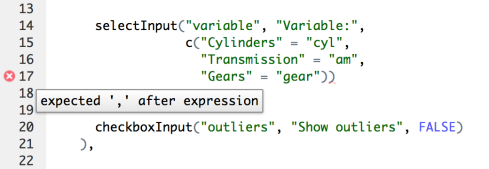
Here the diagnostic indicates that we’ve forgotten a comma within a shiny UI definition:

diagnostics-comma

This diagnostic flags an unknown parameter to a function call:

Screen Shot 2015-04-08 at 11.50.07 AM

This diagnostic indicates that we’ve referenced a variable that doesn’t exist and suggests a fix based on another variable in scope:

Screen Shot 2015-04-08 at 4.23.49 PM

A wide variety of diagnostics are supported, including optional diagnostics for code style issues (e.g. the inclusion of unnecessary whitespace). Diagnostics are also available for several other languages including C/C++, JavaScript, HTML, and CSS.

Configuring Diagnostics

By default, code in the current source file is checked whenever it is saved, as well as if the keyboard is idle for a period of time. You can tweak this behavior using the Code -> Diagnostics options:

diagnostics-options

Note that several of the available diagnostics are disabled by default. This is because we’re in the process of refining their behavior to eliminate “false negatives” where correct code is flagged as having a problem. We’ll continue to improve these diagnostics and enable them by default when we feel they are ready.

Trying it Out

You can try out the new code diagnostics by downloading the latest preview release of RStudio. This feature is a work in progress and we’re particularly interested in feedback on how well it works. Please also let us know if there are common coding problems which you think we should add new diagnostics for. We hope you try out the preview and let us know how we can make it better.


To leave a comment for the author, please follow the link and comment on his blog: RStudio Blog.

R-bloggers.com offers daily e-mail updates about R news and tutorials on topics such as: visualization (ggplot2, Boxplots, maps, animation), programming (RStudio, Sweave, LaTeX, SQL, Eclipse, git, hadoop, Web Scraping) statistics (regression, PCA, time series, trading) and more...
See R in action at the BUILD conference

$
0
0

(This article was first published on Revolutions, and kindly contributed to R-bloggers)

Build 2015, the Microsoft conference which brings around 5,000 developers to the Moscone Center in San Francisco, begins tomorrow. The conference is sold out, but you can livestream the keynote presentations from buildwindows.com to catch all the big announcements. You can also follow along on Twitter at the #Build2015 hashtag.

Build

There will be a major keynote presentation featuring CEO Satya Nadella today (Wednesday) from 8:30AM to 11:00AM Pacific Time. But R users should also be sure to tune in to the keynote tomorrow (Thursday), also from 8:30AM to 11:00AM. I can reveal that R will be a significant component of the presentation by Joseph Sirosh, and will include at around 9:30AM a live demo of Revolution R running in the Azure cloud. I can't reveal all the details yet, but there will be a live demo of distributed big-data computing with R on Azure HDInsights Hadoop using Bioconductor, and Shiny. There will also be several other very cool machine learning applications to see. Don't miss it!

Microsoft Build 2015: Agenda 

To leave a comment for the author, please follow the link and comment on his blog: Revolutions.

R-bloggers.com offers daily e-mail updates about R news and tutorials on topics such as: visualization (ggplot2, Boxplots, maps, animation), programming (RStudio, Sweave, LaTeX, SQL, Eclipse, git, hadoop, Web Scraping) statistics (regression, PCA, time series, trading) and more...

The First NY R Conference

$
0
0

(This article was first published on Revolutions, and kindly contributed to R-bloggers)

by Joseph Rickert

Last Friday and Saturday the NY R Conference briefly lit up Manhattan's Union Square neighborhood as the center of the R world. You may have caught some of the glow on twitter. Jared Lander, volunteers from the New York Open Statistical Programming Meetup along with the staff at Workbench (the conference venue) set the bar pretty darn high for a first time conference.

WorkbenchNYR

The list of speakers was impressive (a couple of the presentations approached the sublime), the venue was bright and upscale, the food was good, and some of the best talks ran way over the time limit but somehow the clock slowed down to sync to the schedule.

But the best part of the conference was the vibe! It was a sweet brew of competency, cooperation and fun. The crowd, clearly out to enjoy themselves, provided whatever lift the speakers needed to be at the top of their game. For example, when near the very end of the second day Stefan Karpinsky's PC just "up and died" as he was about to start his Julia to R demo the crowd hung in there with him and Stefan managed an engaging, ad lib, no visuals 20 minute talk. It was also uncanny how the talks seemed to be arranged in just the right order. Mike Dewar, a data scientist with the New York Times, gave the opening presentation which featured some really imaginative and impressive data visualizations that wowed the audience. But Bryan Lewis stole back the thunder, and the applause, later in the morning when as part of his presentation on htmlwidgets he reproduced Dewar's finale viz with mushroom data.


Bryan has posted his slides on his site here along with a promise to post all of the code soon. 

The slides from all of the presentations have yet to be posted on the NY R Conference website. So, all I can do here today is to provide an opportunity sample drawn from postings I have managed to find scattered about the web. Here are Winston Chang's talk on Dashboarding with Shiny, Jared Lander's talk on Making R Go Faster and BiggerWes McKinney's talk on Data Frames,  my talk on Reproducibility with the checkpoint package, and Max Richman's talk on R for Survey Analysis.

For the rest of the presentations, we will have to wait for the slides to become available on the conference site. There is a lot to look forward to: Vivian Peng's presentation on Storytelling and Data Visualization will be worth multiple viewings and you will not want to miss Hilary Parker's hilarious "grand slam" talk on Reproducible Analysis in Production featuring explainR and complainR. But for sure, look for Andrew Gelman's talk: But When You Call Me A Bayesian I Know I'm Not the Only One. Gelman delivered what was possibly the best technical talk ever, but we will have to wait for the conference video to reassess that. 

GelmanNYR

Was Gelman's talk really the best ever, or was it just the magic of his delivery and the mood of the audience that made it seem so? Either way, I'm glad I was there.

To leave a comment for the author, please follow the link and comment on his blog: Revolutions.

R-bloggers.com offers daily e-mail updates about R news and tutorials on topics such as: visualization (ggplot2, Boxplots, maps, animation), programming (RStudio, Sweave, LaTeX, SQL, Eclipse, git, hadoop, Web Scraping) statistics (regression, PCA, time series, trading) and more...

Dockerizing a Shiny App

$
0
0

(This article was first published on Flavio Barros » r-bloggers, and kindly contributed to R-bloggers)

After a long pause of more than four months, I am finally back to post here. Unfortunately, many commitments prevented me keep posting, but coming back, i changed the deployment (now this blog runs entirely within a docker container with some other cool things I intend to post more forward) and wrote this post.

1. R e apps Shiny

If you are reading this post here, you probably know what Shiny is. OK, but in the case you don’t, you can see it in action! This is the App that i dockerized. Soon you will able to run it at any computer with docker installed.

2. Docker

If you somehow accompanies the open source world news then you probably have heard of Docker. Docker is a fantastic tool for creating software containers, totally isolated from the host operating system. It works like a virtual machine, but it’s much lighter.

The idea behind docker is that the developer creates a container with all dependencies that he wants, make sure that everything works and done. The staff responsible for software deployment does not need to know what is inside the container, it just needs to be able to run container on the server. While this feature could be achieved with virtual machines, they ended up coming with much more than necessary, so the VM files are too large and the host system becomes very slow.

On the other hand, docker does not use a full OS, it shares the same host kernel (yes, it needs to run on Linux) but is a completely isolated environment. So run a docker containers is much lighter than run a virtual machine. Docker features do not stop there, it also allows a kind of versioning and has a kind of github for containers, the Docker Hub, where the user can download and use ready images  for various software, such as MySQL, Postgres , LAMP, WordPress, RStudio, among others. If you want to better understand what is Docker, watch this video.

3. Dockerizing a Shiny app

I just showed you an example of a Shiny app running on RStudio locally. For development it’s ok, but if I want to make it available to anyone? One solution is send the project files. For a basic shiny application just two files are needed (ui.R and server.R).

But what if I want to put on the web? There are two alternatives:

1) A Shiny Server

2) The PaaS shinyapps.io

Option 1) can be very complicated for some users, sometimes not workable, due to the need to install and configure a server.

Option 2) is more interesting, however you it can be expensive, since the free plan can be very limited for some needs.

How docker can help? Initially with the docker you can create a shiny server  using one command. This greatly simplifies deployment of a server. See this short video:

You just need:

docker run --rm -p 3838:3838 rocker/shiny

 WINDOWS AND MAC USERS: You will need boot2docker to reproduce this.

This solution seems to solve the problem. However you can still find several problems such as:

1) How can i put my apps on the server?

2) How can i get a url directly to my app?

3) And this 3838, how can i change it?

4) How can i create an image for my app?

To solve these problems I created a sample container, with a sample app, which appears in the browser as the image is running. Its available at Docker Hub, and it’s ready to test and use. The source code is on Github.

At the following videos i show you how to deploy this app locally and on Digital Ocean. First local:

And on Digital Ocean:

Note that when using the aforementioned command, you do not returns straight to the terminal and you will need a Ctrl + C to close the container. So, to keep the container running and return to the terminal, you should use &.

docker run --rm -p 80:80 flaviobarros/shiny &

You can run this app on Amazon Web Services, Google Cloud and Microsoft Azure, as all of them have support for docker. However, my suggestion is Digital Ocean that is a lot easier to use.

IMPORTANT: through any link to Digital Ocean in this post,  you will earn U$10.00 credit without commitment to keep up the service. With this credit you can keep a simple VPS with 512MB RAM, for two months for free!

The post Dockerizing a Shiny App appeared first on Flavio Barros.

To leave a comment for the author, please follow the link and comment on his blog: Flavio Barros » r-bloggers.

R-bloggers.com offers daily e-mail updates about R news and tutorials on topics such as: visualization (ggplot2, Boxplots, maps, animation), programming (RStudio, Sweave, LaTeX, SQL, Eclipse, git, hadoop, Web Scraping) statistics (regression, PCA, time series, trading) and more...

Shiny: Officer Involved Shootings

$
0
0

(This article was first published on Data Science Las Vegas (DSLV) » R, and kindly contributed to R-bloggers)

US Officer Involved Shootings Mar-Apr 2015 with Shiny

Now everyone can be a data analyst with RStudio’s Shiny package. Fellow R programmer and Las Vegas import, Steve Wells, has created a R-markdown report that shows off some of the features of this dynamic framework.  Using data derived from the Gun Violence Archive and Google maps, interested users can manipulate this data using four different Shiny empowered HTML Widgets from within a single document.

This example of a living article, allows the reader the opportunity to manipulate the data as they peruse it.  Whereas hypertext originally only gave readers reference points (links) within a document, the addition of images illustrated the saying, a picture is worth a thousand words.  The progression from picture to video and other forms of multimedia provided additional levels of meaning. Today it’s applications that give rise to interactive, living articles.

Many technical books are now moving to online, interactive sessions.  Professor Philip B. Stark, chair of Statistics at the University of California Berkley, has delivered his textbook with imbedded videos and sample problems online.  In this way he’s able to fix typos and make updates without having to republish a new edition.  After completing a section, the student is given one or two interactive summary quiz problems which helps solidify the concepts they just learned.  If the student wants more practice they can simply reload the page to get another quiz problem.  These interactive resources create an invaluable feedback loop when learning new concepts.  Now using a combination of Shiny and R-Markdown, a picture becomes an application. These interactive applications provide the ability to gather views that even the original author could not anticipate.

Build Your Own Living Document with Shiny

Steve provides links to each HTML Widget that was used to make the display so that other data analysts can build out their own interactive Shiny reports. Programmers are encouraged to explore further as the complete source code to the Shiny elements are available on github including the scripts used to add Google maps data to the dataset.

The post Shiny: Officer Involved Shootings appeared first on Data Science Las Vegas (DSLV).

To leave a comment for the author, please follow the link and comment on his blog: Data Science Las Vegas (DSLV) » R.

R-bloggers.com offers daily e-mail updates about R news and tutorials on topics such as: visualization (ggplot2, Boxplots, maps, animation), programming (RStudio, Sweave, LaTeX, SQL, Eclipse, git, hadoop, Web Scraping) statistics (regression, PCA, time series, trading) and more...

RStudio v0.99 Preview: Graphviz and DiagrammeR

$
0
0

(This article was first published on RStudio Blog, and kindly contributed to R-bloggers)

Soon after the announcement of htmlwidgets, Rich Iannone released the DiagrammeR package, which makes it easy to generate graph and flowchart diagrams using text in a Markdown-like syntax. The package is very flexible and powerful, and includes:

  1. Rendering of Graphviz graph visualizations (via viz.js)
  2. Creating diagrams and flowcharts using mermaid.js
  3. Facilities for mapping R objects into graphs, diagrams, and flowcharts.

We’re very excited about the prospect of creating sophisticated diagrams using an easy to author plain-text syntax, and built some special authoring support for DiagrammeR into RStudio v0.99 (which you can download a preview release of now).

Graphviz Meets R

If you aren’t familiar with Graphviz, it’s a tool for rendering DOT (a plain text graph description language). DOT draws directed graphs as hierarchies. Its features include well-tuned layout algorithms for placing nodes and edge splines, edge labels, “record” shapes with “ports” for drawing data structures, and cluster layouts (see http://www.graphviz.org/pdf/dotguide.pdf for an introductory guide).

DiagrammeR can render any DOT script. For example, with the following source file (“boxes.dot”):

Screen Shot 2015-04-30 at 12.35.17 PM

You can render the diagram with:

library(DiagrammeR)
grViz("boxes.dot")

grviz-viewer

Since the diagram is an htmlwidget it can be used at the R console, within R Markdown documents, and within Shiny applications. Within RStudio you can preview a Graphviz or mermaid source file the same way you source an R script via the Preview button or the Ctrl+Shift+Enter keyboard shortcut.

This simple example only scratches the surface of what’s possible, see the DiagrammeR Graphviz documentation for more details and examples.

Diagrams with mermaid.js

Support for mermaid.js in DiagrammeR enables you to create several other diagram types not supported by Graphviz. For example, here’s the code required to create a sequence diagram:

sequence

You can render the diagram with:

library(DiagrammeR)
mermaid("sequence.mmd")

sequence-viewer

See the DigrammeR mermaid.js documentation for additional details.

Generating Diagrams from R Code

Both of the examples above illustrating creating diagrams by direct editing of DOT and mermaid scripts. The latest version of DiagrammeR (v0.6, just released to CRAN) also includes facilities for generating diagrams from R code. This can be done in a couple of ways:

  1. Using text substitution, whereby you create placeholders within the diagram script and substitute their values from R objects. See the documentation on Graphviz Substitution for more details.
  2. Using the graphviz_graph function you can specify nodes and edges directly using a data frame.

Future versions of DiagrammeR are expected to include additional features to support direct generation of diagrams from R.

Publishing with DiagrammeR

Diagrams created with DiagrammeR act a lot like R plots however there’s an important difference: they are rendered as HTML content rather than using an R graphics device. This has the following implications for how they can be published and re-used:

  1. Within RStudio you can save diagrams as an image (PNG, BMP, etc.) or copy them to clipboard for re-use in other applications.
  2. For a more reproducible workflow, diagrams can be embedded within R Markdown documents just like plots (all of the required HTML and JS is automatically included). Note that because the diagrams depend on HTML and JavaScript for rendering they can only be used in HTML based output formats (they don’t work in PDFs or MS Word documents).
  3. From within RStudio you can also publish diagrams to RPubs or save them as standalone web pages.

diagrammer-publish

See the DiagrammeR documentation on I/O for additional details.

Try it Out

To get started with DiagrammeR check out the excellent collection of demos and documentation on the project website. To take advantage of the new RStudio features that support DiagrammeR you should download the latest RStudio v0.99 Preview Release.


To leave a comment for the author, please follow the link and comment on his blog: RStudio Blog.

R-bloggers.com offers daily e-mail updates about R news and tutorials on topics such as: visualization (ggplot2, Boxplots, maps, animation), programming (RStudio, Sweave, LaTeX, SQL, Eclipse, git, hadoop, Web Scraping) statistics (regression, PCA, time series, trading) and more...

Introducing Radiant: A shiny interface for R

$
0
0

(This article was first published on R(adiant) news, and kindly contributed to R-bloggers)

Radiant is a platform-independent browser-based interface for business analytics in R, based on the Shiny package.

Key features

  • Explore: Quickly and easily summarize, visualize, and analyze your data
  • Cross-platform: It runs in a browser on Windows, Mac, and Linux
  • Reproducible: Recreate results at any time and share work with others as a state file or an Rmarkdown report
  • Programming: Integrate Radiant’s analysis functions into your own R-code
  • Context: Data and examples focus on business applications

Explore

Radiant is interactive. Results update immediately when inputs are changed (i.e., no separate dialog boxes). This greatly facilitates exploration and understanding of the data.

Cross-platform

Radiant works on Windows, Mac, or Linux. It can run without an Internet connection and no data will leave your computer. You can also run the app as a web application on a server.

Reproducible

Simply saving output is not enough. You need the ability to recreate results for the same data and/or when new data become available. Moreover, others may want to review your analysis and results. Save and load the state of the application to continue your work at a later time or on another omputer. Share state files with others and create reproducible reports using Rmarkdown.

If you are using Radiant on a server you can even share the url (include the SSUID) with others so they can see what you are working on. Thanks for this feature go to Joe Cheng.

Programming

Although Radiant’s web-interface can handle quite a few data and analysis tasks, at times you may prefer to write your own code. Radiant provides a bridge to programming in R(studio) by exporting the functions used for analysis. For more information about programming with Radiant see the programming page on the documentation site.

Context

Radiant focuses on business data and decisions. It offers context-relevant tools, examples, and documentation to reduce the business analytics learning curve.

How to install Radiant

  • Required: R version 3.1.2 or later
  • Required: A modern browser (e.g., Chrome or Safari). Internet Explorer (version 11 or higher) should work as well
  • Recommended: Rstudio

Radiant is available on CRAN. To install the latest version with complete documentation for offline access open R(studio) and copy-and-paste the command below:

install.packages("radiant", repos = "http://vnijs.github.io/radiant_miniCRAN/")

Once all packages are installed use the commands below to launch the app:

library(radiant); radiant("marketing")

See also the Installing Radiant video:

Documentation

Documentation and tutorials are available at http://vnijs.github.io/radiant/ and in the Radiant web interface (the ? icons and the Help menu).

Want some help getting started? Watch the tutorials on the documentation site

Online

Not ready to install Radiant on your computer? Try it online at the links below:

vnijs.shinyapps.io/base

vnijs.shinyapps.io/quant

vnijs.shinyapps.io/marketing

Please send questions and comments to: radiant@rady.ucsd.edu.


aggregated on R-bloggers - the complete collection of blogs about R

To leave a comment for the author, please follow the link and comment on his blog: R(adiant) news.

R-bloggers.com offers daily e-mail updates about R news and tutorials on topics such as: visualization (ggplot2, Boxplots, maps, animation), programming (RStudio, Sweave, LaTeX, SQL, Eclipse, git, hadoop, Web Scraping) statistics (regression, PCA, time series, trading) and more...

Introducing Radiant: A shiny interface for R

$
0
0

(This article was first published on R(adiant) news, and kindly contributed to R-bloggers)

Radiant is a platform-independent browser-based interface for business analytics in R, based on the Shiny package.

Key features

  • Explore: Quickly and easily summarize, visualize, and analyze your data
  • Cross-platform: It runs in a browser on Windows, Mac, and Linux
  • Reproducible: Recreate results at any time and share work with others as a state file or an Rmarkdown report
  • Programming: Integrate Radiant’s analysis functions into your own R-code
  • Context: Data and examples focus on business applications

Explore

Radiant is interactive. Results update immediately when inputs are changed (i.e., no separate dialog boxes). This greatly facilitates exploration and understanding of the data.

Cross-platform

Radiant works on Windows, Mac, or Linux. It can run without an Internet connection and no data will leave your computer. You can also run the app as a web application on a server.

Reproducible

Simply saving output is not enough. You need the ability to recreate results for the same data and/or when new data become available. Moreover, others may want to review your analysis and results. Save and load the state of the application to continue your work at a later time or on another omputer. Share state files with others and create reproducible reports using Rmarkdown.

If you are using Radiant on a server you can even share the url (include the SSUID) with others so they can see what you are working on. Thanks for this feature go to Joe Cheng.

Programming

Although Radiant’s web-interface can handle quite a few data and analysis tasks, at times you may prefer to write your own code. Radiant provides a bridge to programming in R(studio) by exporting the functions used for analysis. For more information about programming with Radiant see the programming page on the documentation site.

Context

Radiant focuses on business data and decisions. It offers context-relevant tools, examples, and documentation to reduce the business analytics learning curve.

How to install Radiant

  • Required: R version 3.1.2 or later
  • Required: A modern browser (e.g., Chrome or Safari). Internet Explorer (version 11 or higher) should work as well
  • Recommended: Rstudio

Radiant is available on CRAN. To install the latest version with complete documentation for offline access open R(studio) and copy-and-paste the command below:

install.packages("radiant", repos = "http://vnijs.github.io/radiant_miniCRAN/")

Once all packages are installed use the commands below to launch the app:

library(radiant); radiant("marketing")

See also the Installing Radiant video:

Documentation

Documentation and tutorials are available at http://vnijs.github.io/radiant/ and in the Radiant web interface (the ? icons and the Help menu).

Want some help getting started? Watch the tutorials on the documentation site

Online

Not ready to install Radiant on your computer? Try it online at the links below:

vnijs.shinyapps.io/base

vnijs.shinyapps.io/quant

vnijs.shinyapps.io/marketing

Please send questions and comments to: radiant@rady.ucsd.edu.


aggregated on R-bloggers - the complete collection of blogs about R

To leave a comment for the author, please follow the link and comment on his blog: R(adiant) news.

R-bloggers.com offers daily e-mail updates about R news and tutorials on topics such as: visualization (ggplot2, Boxplots, maps, animation), programming (RStudio, Sweave, LaTeX, SQL, Eclipse, git, hadoop, Web Scraping) statistics (regression, PCA, time series, trading) and more...

choroplethr v3.1.0: Better Summary Demographic Data

$
0
0

(This article was first published on Just an R Blog » R, and kindly contributed to R-bloggers)

Today I am happy to announce that choroplethr v3.1.0 is now on CRAN. You can get it by typing the following from an R console:

install.packages("choroplethr")

This version adds better support for summary demographic data for each state and county in the US. The data is in two data.frames and two functions. The data.frames are:

  • ?df_state_demographics: eight values for each state.
  • ?df_county_demographics: eight values for each county.

These statistics come from the US Census Bureau’s 2013 5-year American Community Survey (ACS). If you would like the same summary statistics from another ACS you can use these two function:

  • ?get_state_demograhpics
  • ?get_county_demograhpics

For more information on the ACS and choroplethr’s support for it, please see this page.

Relation to Previous Work

In many ways this update is a continuation of work that began with my April 7 guest blog post on the Revolution Analytics blog. In that piece (Exploring San Francisco with choroplethrZip) I explored the demographics of San Francisco ZIP Codes. Because of the interest in that piece, I subsequently released the data as part of the choroplethrZip package. This update simply brings that functionality to the main choroplethr package.

Note that caveats apply to this data. ACS data represent samples, not full counts. I simplify the Census Bureau’s complex framework for dealing with race and ethnicity by dealing with only White not Hispanic, Asian not Hispanic, Black or African American not Hispanic and Hispanic all Races. I chose simplicity over completeness because my goal is to demonstrate technology.

Explore the Data Online

You can explore this data with a web application that I created here. The source code for the app is available here. This app demonstrates some of my favorite ways of exploring demographic data:

  • Using a boxplot to explore the distribution of the data
  • Exploring the data at both the state and county level
  • Using choropleth maps to explore geographic patterns of the data
  • Allowing the user to change the number of colors used:
    • 1 color uses a continuous scale, which makes outliers easy to see
    • Using 2 thru 9 colors puts an equal number of regions in each color. For example, using 2 colors shows values above and below the median

In my opinion, datasets like this really lend themselves to web applications because there are so many ways to visualize the data, and no single way is authoritative.

Selected Images

One of my biggest surprises when exploring this dataset was to discover its strong regional patterns. For example, the regions with the highest percentage White not Hispanic residents tend to be in the north central and north east. The regions with the highest percentage of Black or African American not Hispanic residents is in the south east. And the regions with the highest concentration of Hispanic all Races is in the south west:

state-white

state-black

state-hispanic

Switching to counties shows us the variation within each state. And switching to a continuous scale highlights the outliers.

county-black-continuous

county-hispanic-continuous


To leave a comment for the author, please follow the link and comment on his blog: Just an R Blog » R.

R-bloggers.com offers daily e-mail updates about R news and tutorials on topics such as: visualization (ggplot2, Boxplots, maps, animation), programming (RStudio, Sweave, LaTeX, SQL, Eclipse, git, hadoop, Web Scraping) statistics (regression, PCA, time series, trading) and more...

Extract values from numerous rasters in less time

$
0
0

(This article was first published on R Video tutorial for Spatial Statistics, and kindly contributed to R-bloggers)
These days I was working with a Shiny app for which the computation time is a big problem.
Basically this app takes some coordinates, extract values from 1036 rasters for these coordinates and make some computations. 
As far as I can (and please correct me if I'm wrong!) tell there are two ways of doing this task:
1) load all the 1036 rasters and extract the values from each of them in a loop
2) create a stack raster and extract the values only one time

In the first approach it helps if I have all my rasters in one single folder, since in that case I can run the following code:

f <- list.files(getwd()) 
ras <- lapply(f,raster)
ext <- lapply(ras,extract,MapUTM)
ext2 <- unlist(ext)
t1 <- Sys.time()


The first line creates a list of all the raster file in the working directory, then with the second line I can read them in R using the package raster.
The third line extracts from each raster the values that corresponds to the coordinates of the SpatialPoints object named MapUTM. The object ext is a list, therefore I have to change it into a numeric vector for the computations I will do later in the script.
This entire operation takes 1.835767 mins.

Since this takes too much time I thought of using a stack raster. I can just run the following line to create
a RasterStack object with 1036 layers. This is almost instantaneous.

STACK <- stack(ras)
 
The object looks like this:
> STACK
class : RasterStack
dimensions : 1217, 658, 800786, 1036 (nrow, ncol, ncell, nlayers)
resolution : 1000, 1000 (x, y)
extent : 165036.8, 823036.8, 5531644, 6748644 (xmin, xmax, ymin, ymax)
coord. ref. : NA
names : Dir_10, Dir_11, Dir_12, Dir_13, Dir_14, Dir_15, Dir_16, Dir_17, Dir_18, Dir_19, Dir_20, Dir_21, Dir_22, Dir_23, Dir_24, ...
min values : 59.032657, 141.913933, 84.781970, 147.634633, 39.723591, 154.615133, 45.868360, 197.306633, 85.839959, 272.336367, 93.234409, 339.732100, 79.106781, 566.522933, 175.075968, ...
max values : 685.689288, 2579.985700, 840.835621, 3575.341167, 1164.557067, 5466.193933, 2213.728126, 5764.541400, 2447.792437, 4485.639133, 1446.003349, 5308.407167, 1650.665136, 5910.945967, 2038.332471, ...


At this point I can extract the coordinates from all the rasters in one go, with the following line:
ext <- extract(STACK,MapUTM)
  

This has the advantage of creating a numeric vector, but unfortunately this operation is only slightly faster than the previous one, with a total time of 1.57565 mins

At this point, from a suggestion of a colleague Kirill Müller (http://www.ivt.ethz.ch/people/muelleki), I tested ways of translating the RasterStack into a huge matrix and then query it to extract values.
I encountered two problems with this approach, first is the amount of RAM needed to create the matrix and second is identify the exact row to extract from it.
In the package raster I can transform a Raster object into a matrix simply by calling the function as.matrix. However my RasterStack object has 800786 cells and 1036 layers, meaning that I would need to create a 800786x1036 matrix and I do have enough RAM for that.
I solved this problem using the package ff. I can create a matrix object in R that is associated with a physical object on disk. This approach allowed me to use a minimum amount of RAM and achieve the same results. This is the code I used:

mat <- ff(vmode="double",dim=c(ncell(STACK),nlayers(STACK)),filename=paste0(getwd(),"/stack.ffdata"))
 
for(i in 1:nlayers(STACK)){
mat[,i] <- STACK[[i]][]
}
save(mat,file=paste0(getwd(),"/data.RData"))

With the first line I create an empty matrix with the characteristics above (800786 rows and 1036 columns) and place it on disk.
Then in the loop I fill the matrix row by row. There is probably a better way of doing it but this does the job and that is all I actually care about. finally I save the ff object into an RData object on disk, simply because I had difficulties loading the ff object from disk.
This process takes 5 minutes to complete, but it is something you need to do just once and then you can load the matrix from disk and do the rest.

At this point I had the problem of identifying the correct cell from which to extract all the values. I solved it by creating a new raster and fill it with integers from 1 to the maximum number of cells. I did this using the following two lines:

ID_Raster <- raster(STACK[[1]])
ID_Raster[] <- 1:ncell(STACK[[1]])

Now I can use the extract function on this raster to identify the correct cell and the extract the corresponding values from the ff matrix, with the following lines:

ext_ID <- extract(ID_Raster,MapUTM)
ext2 <- mat[as.numeric(ext_ID),]

If I do the extract this way I complete the process in 2.671 secs, which is of great importance for the Shiny interface.


R code created by Pretty R at inside-R.org

To leave a comment for the author, please follow the link and comment on his blog: R Video tutorial for Spatial Statistics.

R-bloggers.com offers daily e-mail updates about R news and tutorials on topics such as: visualization (ggplot2, Boxplots, maps, animation), programming (RStudio, Sweave, LaTeX, SQL, Eclipse, git, hadoop, Web Scraping) statistics (regression, PCA, time series, trading) and more...

A Link Between topicmodels LDA and LDAvis

$
0
0

(This article was first published on Christopher Gandrud (간드루드 크리스토파), and kindly contributed to R-bloggers)

Carson Sievert and Kenny Shirley have put together the really nice LDAvis R package. It provides a Shiny-based interactive interface for exploring the output from Latent Dirichlet Allocation topic models. If you've never used it, I highly recommend checking out their XKCD example (this paper also has some nice background).

LDAvis doesn't fit topic models, it just visualises the output. As such it is agnostic about what package you use to fit your LDA topic model. They have a useful example of how to use output from the lda package.

I wanted to use LDAvis with output from the topicmodels package. It works really nicely with texts preprocessed using the tm package. The trick is extracting the information LDAvis requires from the model and placing it into a specifically structured JSON formatted object.

To make the conversion from topicmodels output to LDAvis JSON input easier, I created a linking function called topicmodels_json_ldavis. The full function is below. To use it follow these steps:

  1. Create a VCorpus object using the tm package's Corpus function.

  2. Convert this to a document term matrix using DocumentTermMatrix, also from tm.

  3. Run your model using topicmodel's LDA function.

  4. Convert the output into JSON format using topicmodels_json_ldavis. The function requires the output from steps 1-3.

  5. Visualise with LDAvis' serVis.

To leave a comment for the author, please follow the link and comment on his blog: Christopher Gandrud (간드루드 크리스토파).

R-bloggers.com offers daily e-mail updates about R news and tutorials on topics such as: visualization (ggplot2, Boxplots, maps, animation), programming (RStudio, Sweave, LaTeX, SQL, Eclipse, git, hadoop, Web Scraping) statistics (regression, PCA, time series, trading) and more...

Run Shiny app on a Ubuntu server on the Amazon Cloud

$
0
0

(This article was first published on R Video tutorial for Spatial Statistics, and kindly contributed to R-bloggers)
This guide is more for self reference than anything else. 
Since I struggled for two days trying to find all the correct setting to complete this task, gathering information from several websites, I decided to write a little guide on this blog so that if I want to do it again in the future and I do not remember anything (this happens a lot!!) at least I have something to resuscitate my memory.

I found most of the information and code I used from these websites:
http://tylerhunt.co/2014/03/amazon-web-services-rstudio/
http://www.howtogeek.com/howto/41560/how-to-get-ssh-command-line-access-to-windows-7-using-cygwin/
http://www.rstudio.com/products/shiny/download-server/


Preface
First I would like to point out that this guide assumes you (I am talking to myself of the future) remember how to open an instance in the Amazon Cloud. It is not that difficult, you go to this page:
http://aws.amazon.com/ec2/

you log in (if you remember the credentials) and you should see the "Amazon Web Services" page, here you can select EC2 and launch an instance. Remember to select the correct server from the menu on the top right corner since the last time you run all the instances from Oregon, and you live in freaking Switzerland!!


Guide
1) Install Cygwin
This software is needed to communicate with the Ubuntu server.
It is important to follow the instructions on this page (http://www.howtogeek.com/howto/41560/how-to-get-ssh-command-line-access-to-windows-7-using-cygwin/) to install the software correctly.
In particular during the installation process a "select packages" windows appears where we need to select openssh and click on "skip", until there is a cross on the column bin.

When Cygwin is installed we need to click with the right button on the icon and select "run as administrator", then open it.
Now we can run the following line to install ssh:

ssh-host-config

During the process several questions will be asked, the following answers apply:
- Should privilege separation be used? YES
- New local account sshd? YES
- Run ssh as a service? YES
- Enter a value for daemon:  ntsec
- Do you want to use a different name? NO
- Create a new privilege account user? YES  -> then insert a password


After the installation we need to insert the following line to start the sshd service:

net start sshd

Then this line to configure the service:

ssh-user-config

Again it will ask a series of questions. There is a difference between the new version and what is written on the website.
Now it asks only about an SSH2 RSA identity file to be created, the answer is YES.
Then it asks other two questions regarding DSA files and another thing, the answers here are two NO.


2) Connect to the Amazon Server
Open Cygwin.
Go to the folder where the .pem file is saved, using the following line:

cd D:/<folder>/<folder>


NOTE:
Cygwin does not like folder names with spaces!


Now we need to be sure that the .pem key will not be publicly available using the following line

chmod 400 <NAME>.pem

and then we can connect to the ubuntu server using the following line:

ssh -i <NAME>.pem ubuntu@<PUBLIC IP>

These information are provided in Amazon if we click on "Connect" once the instance has properly been launched.
Once we are in we can installing R and Shiny.


3) Install R and Shiny
The first thing to do is set up the root user with the following line:

sudo passwd root

The system will ask to input a password.
Then we can log in using the following line:

su

Now we are logged in as root users.

Now we need to update everything with the following:

apt-get update

At this point we can install R with the following line:

apt-get install r-base


NOTE:
It may be that during the installation process an older version of R is installed and this may create problems with some packages.
To solve this problem we need to modify the file sources.list located in /etc/apt/sources.list
We can do this by using WinSCP, but first we need to be sure that we have access to the folder.
We should run the following two lines:

cd etc/

chmod 777 apt

This gives us access to modify the files in the folder apt via WinSCP (see point 4).

This line of code gives indiscriminate access to the folder, so it is not super secure.

Now we can connect and add the following line at the end:

deb http://cran.stat.ucla.edu/bin/linux/ubuntu trusty/

Then we need to first remove the old version of R using:

apt-get remove r-base

or

apt-get remove r-base-dev

Then we need to run once again both the update and the installation calls.


We can check the amount of disk space left on the server using the following command:

df -h


Then we can start R just by typing R in the console.
At this point we need to install all the packages we would need to run shiny using standard R code:

install.packages("raster")


Now we can exit from R with q() and install shiny suing the following line in ubuntu:

sudo su - -c "R -e "install.packages('shiny', repos='http://cran.rstudio.com/')""

Now we need to install gdebi with the following lines (check here for any update:http://www.rstudio.com/products/shiny/download-server/):

apt-get install gdebi-core
wget http://download3.rstudio.org/ubuntu-12.04/x86_64/shiny-server-1.3.0.403-amd64.deb
gdebi shiny-server-1.3.0.403-amd64.deb


4) Transfer file between windows and Ubuntu
We can use WinSCP (http://winscp.net/eng/index.php) for this task.

First of all we need to import the .pem file that is need for the authentication.
From the "New Site" window we can go to "advanced", then click on "SSH -> Authentication".
From the "Private key file" we can browse and open the .pem file. We need to transform it into a ppk file but we can do that using the default settings.
We can just click on "Save private key" to save the ppk file and then import it again on the same field, and click OK.

Now the Host name is the name of the instance, for example:
ec2-xx-xx-xxx-xxx.eu-west-1.compute.amazonaws.com

The user name is ubuntu and the password is left blank. The protocol is SFTP and the port is 22.

The shiny server is located in the folder /srv/shiny-server

We need to give WinSCP access to this folder using again the command

cd srv
chmod 777 shiny-server


5) Transfer shiny app files on the server
In WinSCP open the folder /srv/shiny-server and create a new folder with the name of your shiny app.
Then transfer the files from your PC to the folder.
Remember to change the address of the files or working directory in the R script with the new links.


6) Allow the port 3838 to access the web
To do this we need to change the rule in the "security groups" menu.
This menu is visible in the main window where all your instances are shown. However, do not access the menu from the panel of the left, that area may be a bit confusing.
Instead select the instance in which you need to add the rule, look at the window at the bottom of the page (the one that shows the name of the instance) and click on the name in light blue near "security group".
This will open the security group menu specific for the instance you selected.
Here we need to add a rule by clicking on "add rule", select custom TCP, write the port number 3838 in the correct area and the select "anywhere" in the IP section.

Now if you go to the following page you should see the app:
<PUBLIC IP>:3838/<FOLDER>


7) Stop, start and restart Shiny server

sudo start shiny-server

sudo stop shiny-server

sudo restart shiny-server


8) Installing rgdal
This package require some tweaks before its installations. On this site I found what I needed: http://askubuntu.com/questions/206593/how-to-install-rgdal-on-ubuntu-12-10

Bascially from the Ubuntu console just run these three lines of code:
sudo apt-get install aptitude
sudo aptitude install libgdal-dev
sudo aptitude install libproj-dev


Then go back to R and install rgdal normally (with install.packages)

To leave a comment for the author, please follow the link and comment on his blog: R Video tutorial for Spatial Statistics.

R-bloggers.com offers daily e-mail updates about R news and tutorials on topics such as: visualization (ggplot2, Boxplots, maps, animation), programming (RStudio, Sweave, LaTeX, SQL, Eclipse, git, hadoop, Web Scraping) statistics (regression, PCA, time series, trading) and more...

In case you missed it: April 2015 roundup

$
0
0

(This article was first published on Revolutions, and kindly contributed to R-bloggers)

In case you missed them, here are some articles from April of particular interest to R users.

Joseph Rickert reviews the inaugural New York City R User Conference, featuring Andrew Gelman.

Engineer Vineet Abraham compares performance benchmarks for R and Revolution R Open on OS X and Ubuntu.

R was featured in the keynotes for the BUILD developer’s conference.

Mark Malter created a Shiny application to explore baseball statistics.

A curated list of the best packages, add-ons and resources for R according to Qin Wenfeng.

An analysis of paintings from British museums reveals an increasing use of the colour blue over the last two centuries.

Journalists are increasingly referencing source research via DOIs, and packages from rOpenSci allow R users to access that research programmatically.

Microsoft is hiring programmers to work on R-related projects.

Some examples of visualizing the results of hierarchical clustering with a heat map.

The Financial Times published an interactive data visualization based on R to explore European unemployment statistics.

Announcing R 3.2.0.

Recent R user group meetings have covered Shiny, SparkR, htmlwidgets, and dynamic pricing models.

A story about teaching R to archaeologists in Myanmar, and coping with package installation in a low-bandwidth environment with the miniCRAN package.

RPowerLabs allows electrical engineers to experiment on virtual power distribution systems.

Two high-performance packages from RStudio for reading data into R: readr (for text data) and readxl (for Excel data).

A list of the top 25 R user groups in the world by membership.

A guide to association rules and market basket analysis in R.

The choroplethrZip package allows R users to create data maps from US zip codes.

Revolution Analytics is now a subsidiary of Microsoft.

DeployR 7.4, a web-services framework for integrating R code to other applications, is now available for download.

Coarse-grained parallel computing with R on servers and Hadoop with rxExec in Revolution R Enterprise.

Revolution R Open 8.0.2 was released (and RRO 8.0.3 is now available, too).

General interest stories (not related to R) in the past month included: a video travelling at the speed of light, a snowy music video, and visualizing the bassline in a Marvin Gaye classic.

As always, thanks for the comments and please send any suggestions to me at david@revolutionanalytics.com. Don't forget you can follow the blog using an RSS reader, via email using blogtrottr, or by following me on Twitter (I'm @revodavid). You can find roundups of previous months here.

To leave a comment for the author, please follow the link and comment on his blog: Revolutions.

R-bloggers.com offers daily e-mail updates about R news and tutorials on topics such as: visualization (ggplot2, Boxplots, maps, animation), programming (RStudio, Sweave, LaTeX, SQL, Eclipse, git, hadoop, Web Scraping) statistics (regression, PCA, time series, trading) and more...
Viewing all 673 articles
Browse latest View live


Latest Images